10. Gas Power Cycles - Brayton, Otto and Diesel Cycles#
In the last two chapters, the concepts of heat engines (Section 8.7 Heat Engines), thermal efficiency (Section 8.7.1 Heat Engine Thermal Efficiency), isentropic efficiency (Section 9.4 Isentropic Efficiency) were introduced in a relatively general way. The Carnot heat engine was introduced as the idealized and reversible heat engine with the maximum theoretical efficiency operating between two thermal reservoirs. In this chapter and the next, a variety of operational strategies for real heat engines will be discussed, some based on open system components that produce shaft work with a turbine and some as a series of piston expansion/compression processes.
Heat engines, or power cycles, can be generally categorized as either gas power cycles or vapor power cycles. The distinction between the two is the working fluid. In the case of gas power cycles, the working fluid is a gas, typically air, which does not undergo a change in phase. Vapor power cycles, on the other hand, utilize a working fluid such as H2O that undergoes phases change during the cycle. In this chapter the focus is gas power cycles, and next chapter will focus on vapor power cycles.
The gas power cycles to be discussed in this chapter are the Brayton Cycle, Otto Cycle, Diesel Cycle, Striling Cycle and Ericsson Cycles. The former is the gas power cycle that utlizes turbine and compressor technology and is the heart of many power plants and jet engines. The latter are all based on piston cylinder designs where the Otto and Diesel are the main internal combustion engine technologies and the Stirling and Ericcson Cycles integrate heat recuperation for high theoretical efficiencies and are externally heated.
10.1. Brayton Power Cycle#
The Brayton Power Cycle is at the heart of many power plants and jet engines and utilizes turbomachinery, such as gas turbines and compressors, to perform mechanical shaft work. The real and open-system Brayton power cycle is composed of a compressor, combustor and gas turbine, as seen below in Figure 10.1. Fresh air enters the compressor, is compressed (process 1-2), combusted at high pressure (process 2-3) with a fuel to produce heat, resulting in combusion products that are expanded in a gas turbine to produce shaft work (process 3-4). The surrounding air serves as a heat sink for the thermal energy disspated from the combusion products. As drawn, this Brayton cycle may be considered an open system when taken as a whole, with fresh air enetering the control volume and combustion products leaving.

Fig. 10.1 A schematic of an open and real Brayton Power Cycle. Fresh air is fed to the system, compressed, combusted with a fuel, followed by expansion of the combustion products in a turbine to produce shaft work.#
10.1.1. Ideal Brayton Power Cycle#
There are several simplifying assumptions that are typically made to decrease the complexity of the Brayton cycle without sacrificing greatly the accuracy. The first and main assumption is referred to as the air-standard assumption. In this case, the working fluid is approximated as air as an ideal gas that flows in a closed-loop cycle, where it is compressed, heated externally with a high temperature heat exchanger, expanded in a turbine and cooled in a heat exchanger to complete the cycle. Another assumption is that both the compression and expansion processes are reversible and adiabatic (i.e. isentropic). A thired assumption is that the heat addition and rejection in the high and low temperature heat exchangers occurs at constant pressure. And finally, the entire process is assumed to operate at steady state. This Ideal Brayton Cycle is shown below in Figure 10.2. To simplify analysis further, sometimes a cold-air approximation may be used which assumes constant specific heats, both cp and cv of air at ambient conditions, and all prior equations that assume constant specific heats may be applied, such as those from Section 9.2 Isentropic Processes of Ideal Gases. Finally, real turbines and compressors may be analyzed within the framework of this cycle by accounting for their isentropic efficiencies, as discussed in Section 9.4 Isentropic Efficiency.

Fig. 10.2 An example of a closed and ideal Brayton Cycle. Air is circulated in a closed loop, where it is first compressed isentropically, heated at constant pressure in a heat exchanger, expanded isentropically to produce shaft work, and finally cooled at constant pressure in a low temperature heat exchanger.#
With an appropriate system boundary around every component, this can be treated as a closed system, and analyzed with the closed system energy balance equation, in rate form, discussed in Section 5.2 Energy Transfer and The First Law.
Because the process operates at steady state, \(\frac{dU}{dt} = 0\), and
The thermal efficiency is then
When an appropriate boundary is drawn around a component of interest within the cycle, it should be analyzed with the steady state open system energy balance discussed in Section 7 First Law of Thermodynamics - Open Systems. Using this form of the energy equation enables determination of either desired heat transfer rates and work terms, or it can be used to evaluate appropriate state properties at the inlets or exits. For example, taking the turbine as the control volume and assuming steady state, adiabatic, negligible change in kinetic and potential energies, the energy equation becomes the following.
Recognizing that state 3 is the inlet and state 4 is the exit it can also be written as below.
And if specific heats are used, then either average specific heat or using cold-air approximation may be used, understanding the assumptions inherent to each approach.
Note that if average values for specific heats are used and one of the temperatures are not known, then an iterative, or guess and check solution approach would be required. Refer to Section 9.4.2 Example - Isentropic Efficiency Iterative Solution Approach as an example.
10.1.1.1. Example - Analysis of an Ideal Brayton Cycle#
In a Brayton cycle, air enters the compressor at 0.1 MPa and 298 K. The pressure leaving the compressor is 1.0 MPa and the maximum temperature is 1240 K. Assume an isentropic efficiency of 80% for the compressor and 85% for the turbine. Determine the compressor specific work, turbine specific work and cycle efficiency. Use property values from Cantera (i.e. variable specific heats) rather than constant specific heat equations. Understand how to solve using constant specific heat equations.
Solution There are only two pressures in this simple Brayton cycle, and thus all pressures are known. The maximum temperature occurs after external heat addition, and therefore the only properties not given are the temperatures following compression and expansion. We can use the provided isentropic efficiencies to determine enthalpies at each of these states. For this we will need to recognize that the entropy at the inlet and exit of the compressor and turbine are equal in the isentropic case.
import cantera as ct
#we have 6 total states including the isentropic states, thus we will set each of these to be air

state1,state2s,state2,state3,state4s,state4 = ct.Solution('gri30.yaml'),ct.Solution('gri30.yaml'),ct.Solution('gri30.yaml'),ct.Solution('gri30.yaml'),ct.Solution('gri30.yaml'),ct.Solution('gri30.yaml')
state1.X,state2s.X,state2.X,state3.X,state4s.X,state4.X = 'N2:0.79 O2: 0.21','N2:0.79 O2: 0.21','N2:0.79 O2: 0.21','N2:0.79 O2: 0.21','N2:0.79 O2: 0.21','N2:0.79 O2: 0.21'

#given or inferred properties
p1 = 0.1*10**6 #Pa
p4=p1 #constant pressure heat rejection
T1 = 298 #K
p2 = 1*10**6 #Pa
p3=p2 #constant pressure heat addition
T3 = 1240 #K
eta_comp = 0.8
eta_turb = 0.85

#determine s1 and equate to s2s
state1.TP = T1,p1
s1 = state1.SP[0]
s2s=s1
#also we can get h1
h1 = state1.HP[0]

#knowing s2s and p2, determine h2s
state2s.SP = s2s,p2
h2s = state2s.HP[0]

#solve for h2 using isentropic efficiency of the compressor
h2 = (h2s-h1)/eta_comp+h1

print ("specific enthalpies at states 1 and 2 are ", round(h1,2), "and", round(h2,2), "kJ kg-1")
specific enthalpies at states 1 and 2 are -112.33 and 348170.44 kJ kg-1
#determine s3 and equate to s4s
state3.TP = T3,p3
s3 = state3.SP[0]
s4s=s3
#also we can get h3
h3 = state3.HP[0]

#knowing s4s and p4, determine h4s
state4s.SP = s4s,p4
h4s = state4s.HP[0]

#solve for h4 using isentropic efficiency of the turbine
h4 = h3-(h3-h4s)*eta_comp

print ("specific enthalpies at states 3 and 4 are ", round(h3,2), "and", round(h4,2), "J kg-1")
specific enthalpies at states 3 and 4 are 1034042.51 and 533284.7 J kg-1
Now it is a matter of performing energy balances for the compressor, turbine and high temperature heat exchanger. Assuming steady state operation, adiabatic, negligable kinetic and potential energies, the open system energy conservation equation reduces to the follwoing specific work terms for each.
\( w_{\rm 12} = (h_{\rm 1}-h_{\rm 2})\)
\( w_{\rm 34} = (h_{\rm 3}-h_{\rm 4})\)
Assuming steady state operation, constant pressure, negligable kinetic and potential energies, the open system energy conservation equation reduces to the following specific heat transfer term.
\( q_{\rm 23} = (h_{\rm 3}-h_{\rm 2})\)
Each of the specific enthalpy terms has already been determined, so we can solve for each directly.
w_comp = h1-h2
w_turb = h3-h4
q_23 = h3-h2

print("specific compressor work is", round(w_comp/1000,2), "kJ kg-1")
print("specific turbine work is", round(w_turb/1000,2), "kJ kg-1")
print("specific heat transfer is", round(q_23/1000,2), "kJ kg-1")
specific compressor work is -348.28 kJ kg-1
specific turbine work is 500.76 kJ kg-1
specific heat transfer is 685.87 kJ kg-1
Understanding that the thermal efficiency is the net work divided by the heat addition it can be solved directly.
eta_th = (w_comp+w_turb)/q_23

print("The thermal efficiency of the Brayton cycle is", round(eta_th*100,2), "%")
The thermal efficiency of the Brayton cycle is 22.23 %
10.2. Brayton Power Cycle with Intercooling, Reheating and Regeneration#
There are several strategies empolyed to increase the efficiency of the idealized Brayton cycle. These include integrating intercooling, reheating and regeneration strategies. These strategies serve to 1) decrease compression work by integrating cooling during compression, 2) increase turbine work by integrating heat addition during expansion and 3) decrease the amount of external heat transfer required to the system by recuperating heat internally between the exits of the turbine and compressors.
10.2.1. Intercooling#
Last chapter in the section on reversible work, Section 9.3 Reversible Steady State Work, we saw that isentropic compression/expansion does not result in the minimum/maximum shaft work associated with compressors and turbines. Instead, it was shown that isothermal compression and isothermal expansion enable the minimum/maximum work. Thus, compression should be integrated with cooling and expansion with heating, both of which minimuze/maximize volume-pressure relationship correlated with reversible shaft work, shown again below for reference.
In practice, rather than simultaneously cooling during comprssion, intercoolers are utilized between stages of adiabatic compression to intermittantly cool the compresssed gas. The intercooler is simply a gas heat exchanger that rejects heat from the compressed gas at constant pressure. In theory, given a large enough number of compression, intercooling stages, the compression process would approximiate an isothermal process and approach the theoretical minimum work limit. However, for practical considerations, usually no more than a few intercoolers are integrated with the compression process, and there are diminishing returns for each additional intercooler integrated. A schematic of an intercooler integrated between two stages of adiabatic compression, alongside the corresponsing T-s diagram, are shown below in Figure 10.3. As seen, the first compression stage to an intermediate pressure increases temperature and specific volume (not shown). Cooling the gas in an intercooler back to a lower temperature (usually the same as state 1), enables compression to the final pressure at smaller specific volumes compared to the compression process without intercooling, thus reducing \(w_{\rm rev} = - \int vdp\). Also, note that the final temperature is equal to the intermediate temperature(T4 = T2) and is lower than it would be when compared to the compression process without intercooling (T4 > T2), thus better approximating an isothermal compression process.

Fig. 10.3 An intercooler integrated between two stages of adiabatic compression. The intercooler rejects heat from the compressed gas, thereby reducing the amount of compression work required to operate between two pressures.#
10.2.2. Reheating#
Similar to intercooling, reheaters are integrated bewteen stages of adiabatic expansion to approximate isothermal expansion, rather than heating simultaneously during gas expansion. Reheaters are simply gas heat exchangers that supply heat at constant pressure. A schematic of a reheater integrated between two stages of adiabatic expansion, alongside the corresponsing T-s diagram, are shown below in Figure 10.4. As seen, the first expansion stage to an intermediate pressure decreases temperature and specific volume (not shown). Reheating the gas in a reheater back to a higher temperature (usually the same as state 1), enables expansion to the final pressure at larger specific volumes compared to the expansion process without reheating, thus increasing \(w_{\rm rev} = \int vdp\). Also, note that the final temperature is equal to the intermediate temperature(T4 = T2) and is higher than it would be when compared to the compression process without reheating (T4 < T2), thus better approximating an isothermal expansion process.

Fig. 10.4 A reheater integrated between two stages of adiabatic expansion. The reheater supplies heat to the gas at intermediate pressure, thereby increasing the amount of expansion work extracted between high and low pressures.#
An idealized Brayton cycle with intercooling and reheating is shown below in Figure 10.5, alongside a corresponding T-s diagram. As seen, there are three total pressures in this configuration, because intercooling and reheating are typically performed at the same intermediate pressure. The gray dashed line is included only for visualization purposes.
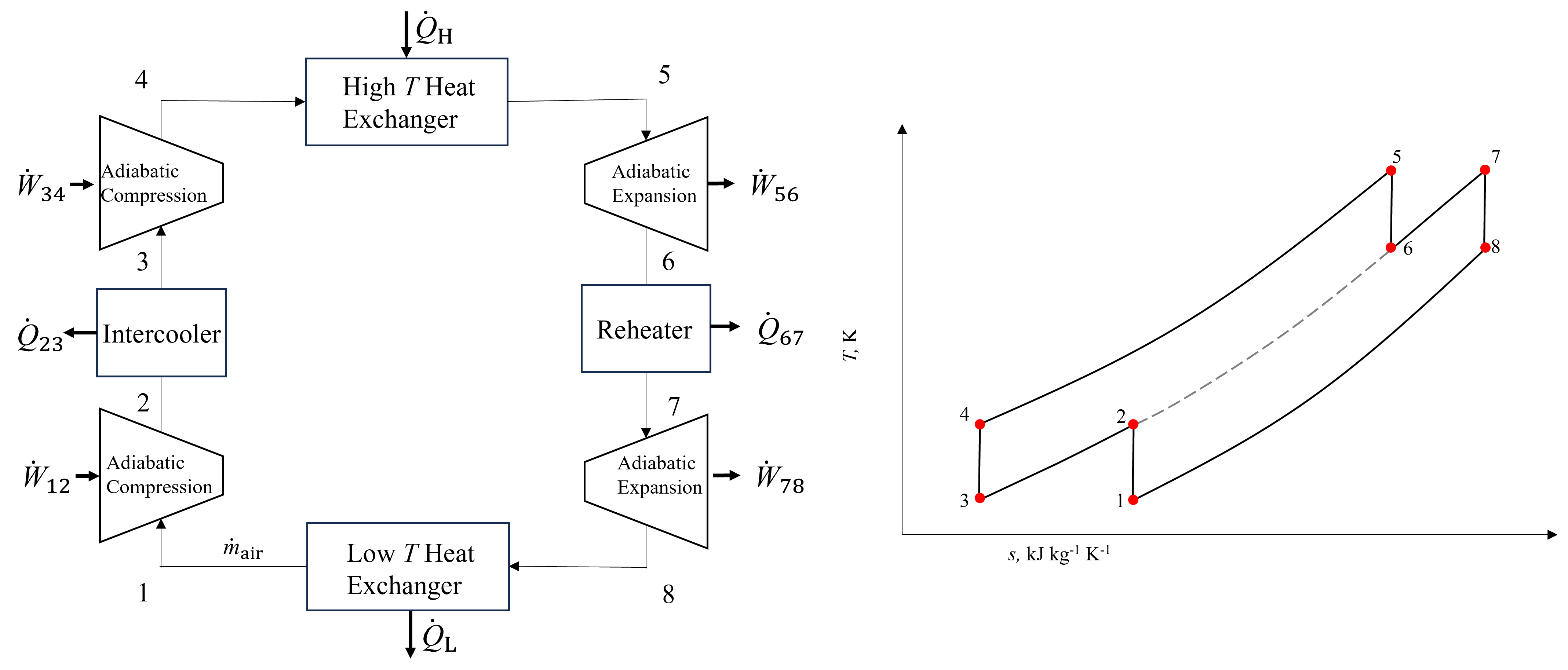
Fig. 10.5 A Brayton cycle with both intercooling and reheating. There are three unique pressures in the cycle because typically intercooling and reheating are performed at the same intermediate pressure.#
10.2.3. Regeneration#
As seen in Figure 10.5, the temperature leaving the low pressure turbine prior to heat rejection (state 8), is greater than the temperature leaving the high pressure compressor prior to external heat addition (state 4). This presents an opportunity to integrate internal heat recupertation between these two different temperature streams, in order to reduce the external heat addition requirement and thus boost efficiency. The heat exchanger responsible for this internal heat recuperation is called a regenerator. An example of a Brayton cycle incorporating an intercooler, reheater and regenerator is shown below in Figure 10.6. The regenerator is a counterflow heat exchanger that operates at constant pressure and is designed to transfer the relatively high temperature heat leaving the low pressure turbine to the exit of the high temperature compressor.
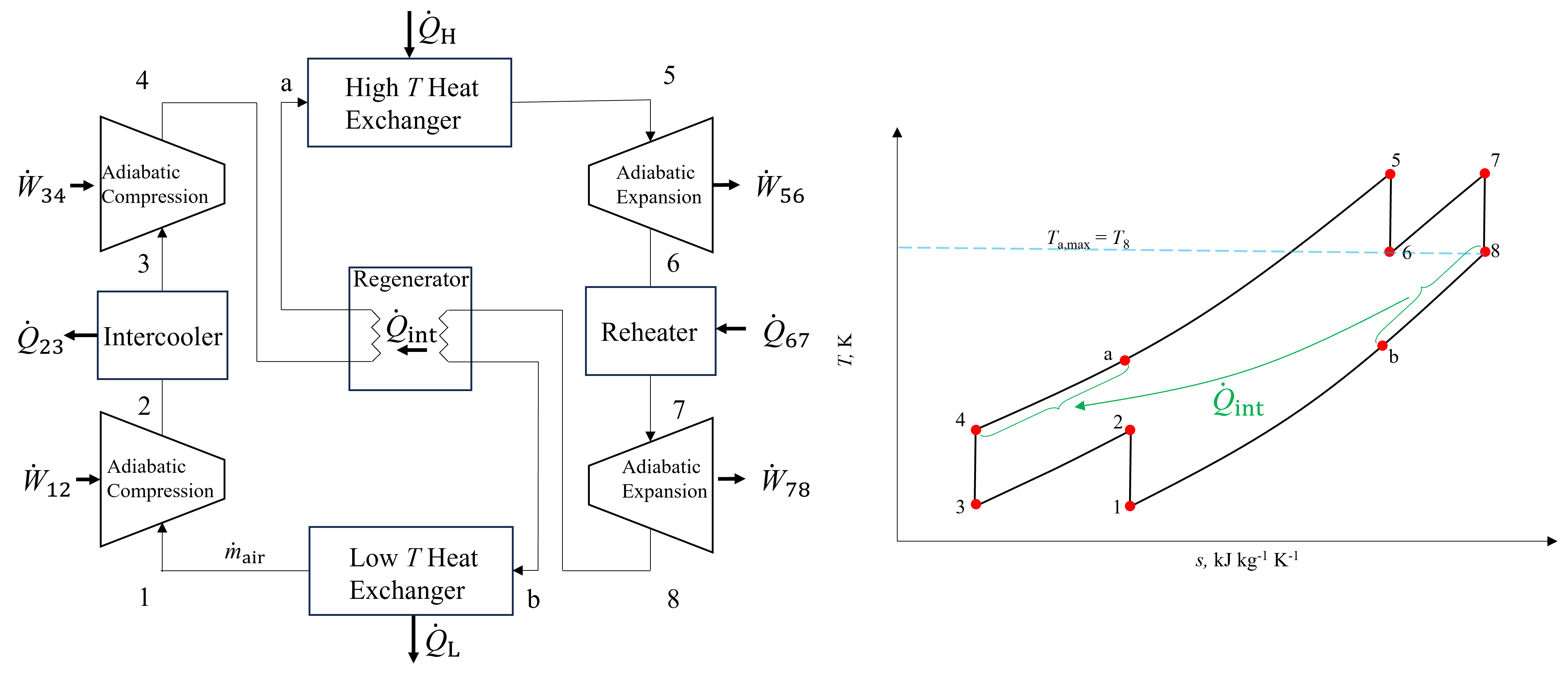
Fig. 10.6 A Brayton cycle with both intercooling, reheating and regeneration. There are three unique pressures in the cycle because typically intercooling and reheating are performed at the same intermediate pressure. The maximim temperature leaving the cold stream is the temperature entering on the hot side, at state 8.#
The resulting state following heat addition to the cold temperature side is labled state a, and from the high temperature side, state b. As seen, because both the hot and cold gases in the heat exchanger exchange heat at constant pressure, there is no change in the T-s diagram compared to a process without the regenerator, with the exception of the added states a and b. The regenerator may be analyzed as an open system and adiabatic heat exchanger with two inlets and two exits operating at steady state. Ignoring changes in kinetic and potential energies of the fluids and disregarding any work terms, the energy conservation equation reduces to the form below.
Thus, the change in enthalpy of the hot stream leaving the turbine is equal to the enthalpy gain in the cold stream.
The enthalpy change of each stream is also the amount of heat internally recuperated, \(\dot Q_{\rm int}\). This amount of heat recuperation directly reduces the amount of external heat required to heat to the inlet temperature of the high pressure turbine, state 5, which in specific temrms is equal to \(h_{\rm 5}-h_{\rm a}\).
To determine state properties exiting the regenerator, it is not sufficient to only apply an open system energy balance around the heat exchanger because both temperatures are usually unknown. To resolve this, the of the heat exchanger is required. Effectivness (\(\epsilon_{\rm reg}\)), or heat exchanger effectiveness factor, is a measure of the real heat exchanger performance relative to the maximum possible, and. The maximum possible performance is determined by recognizing that the maximum temperature that the cold fluid could be heated to is the the exit temperature of the low pressure turbine at state 8. This can be imagined by a counterflow heat exchanger where there is an infintesimally small temperature difference between hot and cold streams at each position within the heat exchanger. If it were any higher then this would violate the second law of thermodynamics because heat cannot be transferred from low to high temperature spontaneously. Mathematically, \(\epsilon_{\rm reg}\) is described as below and is always a value between 0 and 1.
10.2.3.1. Example - Analysis of an Intercooling, Reheating and Regeneration Brayton Cycle#
Consider an ideal gas turbine cycle using air with two stages of isentropic compression and two stages of isentropic expansion. The pressure ratio across each compressor and turbine is 8. Pressure entering the first compressor is 100 kPa, the temperature entering each compressor is 20 °C, and the temperature entering each turbine is 1100 °C. A regenerator is also incorporated with an efficiency of 70%. Determine the specific compressor power input, the specific power output from the turbine and the overall thermal efficiency. Use constant specific heats at @ 300 K – understand how to solve without using specific heats.
Solution For this problem we can take advantage of the isentropic equations to evaluate the compressors and turbines, introduced in Section 9.2 Isentropic Processes of Ideal Gases. We can use these because we are assuming constant specific heats. Since we know inlet and exit temperatures and pressure ratios the form \(\frac{T_2}{T_1} = (\frac{p_2}{p_1})^{\frac{k-1}{k}}\) will be most useful.
import cantera as ct

# first, lets determine k and cp for air at 300 K. We will use 1 bar pressure
#but since air is an ideal gas where specific heats are functions of tmeperature only
#our choice of pressure is irrelevant

state1 = ct.Solution('gri30.yaml')
state1.X = 'N2:0.79 O2: 0.21'
state1.TP = 300,100*10**3 # K,Pa
cp=state1.cp
cv=state1.cv
k = cp/cv
print("cp is", round(cp,2), "kJ kg-1 K-1 and k is", round(k,2))
cp is 1010.07 kJ kg-1 K-1 and k is 1.4
# below is the information given in the problem statement

p_ratio = 8
T1 = 20 +273.15 #K
T3=T1
T5 = 1100+273.15 #K
T7 = T5
eta_reg = 0.7
# analyzing the first compressor we can solve for the exit temperature

T2 = T1*p_ratio**((k-1)/k)

# since the pressure ratio is the same and air is cooled back to 20 C, T4 must be equivilent to T2

T4=T2

print("The compressor exit temperatures are both", round(T2,2), "K")
The compressor exit temperatures are both 530.59 K
# analyzing the first turbine we can solve for the exit temperature

T6 = T5*(1/p_ratio)**((k-1)/k)

# since the pressure ratio is the same and air is heated back to 1100 C, T8 must be equivilent to T6

T8=T6

print("The turbine exit temperatures are both", round(T6,2), "K")
The turbine exit temperatures are both 758.67 K
# analyzing the regenerator, the max temperature exiting the cold stream is T8

Tmax = T8
Ta = T4+eta_reg*(Tmax-T4)
print("The regenerator exit temperatures on the cold side is", round(Ta,2), "K")
The regenerator exit temperatures on the cold side is 690.24 K
# specific compressor power input

w_12 = cp*(T1-T2)
w_34 = cp*(T3-T4)
w_comp = w_12+w_34
print("The compressor specific work input is", round(w_comp,2), "kJ kg-1")
The compressor specific work input is -479656.17 kJ kg-1
# specific turbine power output

w_56 = cp*(T5-T6)
w_78 = cp*(T7-T8)
w_turb = w_56+w_78
print("The turbine specific work output is", round(w_turb,2), "kJ kg-1")
The turbine specific work output is 1241340.91 kJ kg-1
# To determine efficiency we need to know the external heat addition, heating from
# state a to state 5 and from state 6 to state 7

q_a5 = cp*(T5-Ta)
q_67 = cp*(T7-T6)
q_in = q_a5+q_67
print("The specific heat input is", round(q_in,2), "kJ kg-1")
The specific heat input is 1310453.58 kJ kg-1
# And using the definition of thermal efficiency we can calculate it directly

eta_th = (w_comp+w_turb)/q_in
print("The thermal efficiency is", round(eta_th*100,2), "%")
The thermal efficiency is 58.12 %
Note how much higher this efficiency is compared to the prior example that didn’t incorporate intercooling, reheating and regeneration. We can also see how the efficiency would compare if we were to remove the regenerator by re-calculating the external heat addition from state 4 to 5 and 6 to 7.
q_45 = cp*(T5-T4)
q_67 = cp*(T7-T6)
q_in = q_45+q_67
eta_th = (w_comp+w_turb)/q_in
print("The thermal efficiency without regeneration is", round(eta_th*100,2), "%")
The thermal efficiency without regeneration is 51.75 %
10.3. Closed-System Power Cycles#
Several gas power cycles can be modeled as a series of piston-cylinder expansion/compression processes. Like with the Brayton cycle, air-standard assumptions are often utilized and used exclusively here, rather than accounting for variation in gas species due to combusion processes. These cycles include internal combustion engines, namely the Otto and Diesel cycles, and external combusion engines that incorporate internal heat recuperation to improve efficiency, namely the Stirling and Ericcson cycles.
10.3.1. Otto Cycle#
The Otto cycle, also known as the ideal cycle for spark ignition engines, is typically composed of four complete strokes of a piston within a cylinder. The first two are related to compression and expansion and are closely related to the net work output, whereas the last two are necessary to exhaust combustion products and intake fresh air. The complete analysis, taking into account all four strokes and variation in gas composition, is beyond the scope of this textbook. Nevertheless, a brief explanation and description of the real process is presented. The first stroke consists of compression of air-fuel mixture to a pressure below the auto ignition point, to prevent spontaneous and uncontrolled combustion. This is referred to as the compression stroke. Once sufficiently compressed, the combustion reaction is initiated with a spark (i.e. spark plug), generating heat and increasing pressure. The resulting high pressure combustion gases force the piston down to complte the second stroke, producing useful work output. This is referred to as the power, or expansion stroke. This is followed by an exhaust stroke (third stroke) responsible for removing combustion products through an exhaust valve which are slightly higher than ambient pressure, and finally by an intake stroke (fourth stroke) where fresh air is introduced through an intake valve at slightly less than ambient pressure. Becuase combustion occurs within the piston-cyclinder, the Otto cycle is a type of internal combusion engine.
This four stroke process is greatly simplified using air-standard assumptions. Using air-standard assumptions, the Ideal Otto cycle consists of four internally reversible processes and two piston strokes. Because air standard assumptions are used, the heat transfer occurs from/to and external reservoir. The four processes can be summarized as:
Isentropic compression
Constant volume heat addition from an external source
Isentropic expansion
Constant volume heat rejection
A piston-cylinder representation of the air-standard Ideal Otto Cycle is shown below in Figure 10.7. Starting on the left at state 1, compression work (\(W_{\rm 12}\)) is done to the piston to move it from the bottom dead volume (BDV) to top dead volume (TDV) isentropically. Then, heat is added (\(Q_{\rm 23}\)) from an external source while the piston-cylinder volume remains constant. This results in an increase in temperature and pressure. Following heat addition, the piston expands back to BDV, doing work to the surroundings (\(W_{\rm 34}\)), resulting in a temperature decrease of the air. Finally, the air is further cooled by rejecting heat at constant volume to an external source, going from state 4 to state 1. Notice from the figure that there are only two different volumes throughout the cycle. Also, because both work processes are isentropic, their are only two unique entropies in the cycle. Because heat addition occurs while the volume is held constant, there is by definition no boundary work corresponding to processes 2-3 and 4-1. And because the expansion and compression processes are isentropic and reversible, they must be adiabatic. Thus, there is no heat transfer associated with processes 1-2 and 3-4.
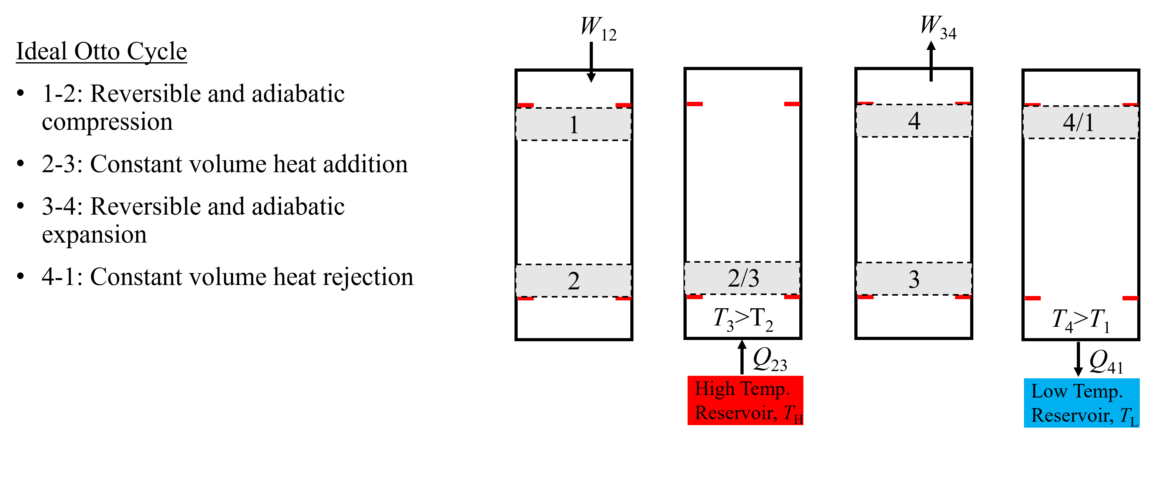
Fig. 10.7 An Ideal Otto Cycle, composed of two piston strokes and 4 unique states.#
It is useful to visualize the Otto Cycle using both a T-s and p-v disgram to understand where all of the work and heat transfer processes are occuring. These are shown below in Figure 10.8. Going from state 1 to state 2, notice on the T-s diagram that the isentropic work process consists of a vertical line increasing in temperature, whereas on the p-v diagram the volume decreases from BDC to TDC. As heat is added during process 2-3, temperature increases as would be expected keeping volume constant, and notice on the p-v diagram this results in a vertial line corresponding to an increase in pressure. Expansion during process 3-4 is isentropic, corresponding to a vertical line decreasing in temperature as seen on the T-s diagram and increase in volume and corresponding decrease in pressure as seen on the p-v diagram. Finally, as heat is rejected, both temperature and entropy decrease, as well as pressure.
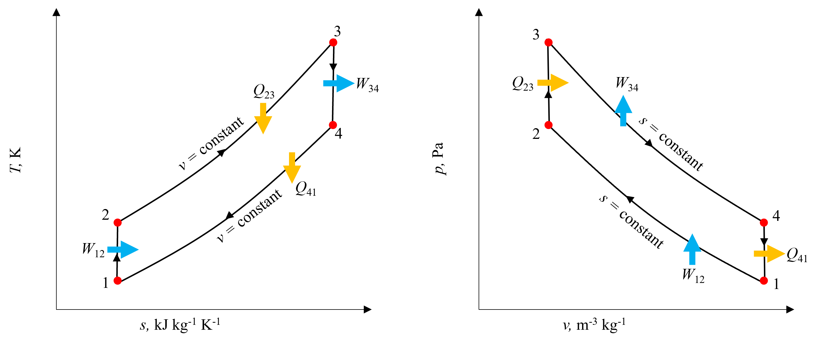
Fig. 10.8 T-s and p-v diagrams for the Ideal Otto Cycle, indicating all relevent heat transfer and work terms, as well as isentropic and isochoric processes.#
Analysis of each of the processes within the Ideal Otto cycle may be performed using the closed system energy conservation equation (Section 5.2 Energy Transfer and The First Law), ideal gas law (Section 4.2 Ideal Gas Equation of State), and when applicable the isentropic ideal gas equations from (Section 9.2 Isentropic Processes of Ideal Gases). Starting from the closed system energy conservation equation (\(\Delta U = 0 = Q_{\rm net} - W_{\rm net}\)) for each process, the following equations can be derived.
Process 1-2: \(\Delta U_{\rm 1-2} = Q_{\rm 1-2} - W_{\rm 1-2}\), where \(Q_{\rm 1-2} = 0\)
thus \(W_{\rm 1-2} = U_{\rm 1} - U_{\rm 2} = m(u_{\rm 1} - u_{\rm 2}) = mc_{\rm v}(T_{\rm 1} - T_{\rm 2})\)
Process 2-3: \(\Delta U_{\rm 2-3} = Q_{\rm 2-3} - W_{\rm 2-3}\), where \(W_{\rm 2-3} = 0\)
thus \(Q_{\rm 2-3} = U_{\rm 3} - U_{\rm 2} = m(u_{\rm 3} - u_{\rm 2}) = mc_{\rm v}(T_{\rm 3} - T_{\rm 2})\)
Process 3-4: \(\Delta U_{\rm 3-4} = Q_{\rm 3-4} - W_{\rm 3-4}\), where \(Q_{\rm 3-4} = 0\)
thus \(W_{\rm 3-4} = U_{\rm 3} - U_{\rm 4} = m(u_{\rm 3} - u_{\rm 4}) = mc_{\rm v}(T_{\rm 3} - T_{\rm 4})\)
Process 4-1: \(\Delta U_{\rm 4-1} = Q_{\rm 4-1} - W_{\rm 4-1}\), where \(Q_{\rm 4-1} = 0\)
thus \(Q_{\rm 4-1} = U_{\rm 1} - U_{\rm 4} = m(u_{\rm 1} - u_{\rm 4}) = mc_{\rm v}(T_{\rm 1} - T_{\rm 4})\)
As seen, each heat transfer and work term associated with each process can be related to the change in internal energy (or temperature using \(c_{\rm v}\)). Note that this is in contrast to the Brayton Cycle analysis where the heat transfer and work terms are related to changes in enthalpy (or temperature using \(c_{\rm p}\)). The use of \(c_{\rm p}\) and \(c_{\rm p}\) depends only on whether changes in enthalpy or energy are of interest, regardless of the process being constant volume, pressure, etc. This is because of our assumption that air is an ideal gas, in which case specific heats are a function of only temperature and the meaning of the constant pressure or volume substripts is no lnger relevent. Refer to Section 6.4 Using Specific Heats with Ideal Gases for more discussion.
For the isentropic compression and expansion processes we can use any of the isentropic equations:\(\frac{T_2}{T_1} = (\frac{v_1}{v_2})^{k-1}\), \(\frac{T_2}{T_1} = (\frac{p_2}{p_1})^{\frac{k-1}{k}}\), or \(\frac{p_2}{p_1} = (\frac{v_1}{v_2})^{k}\). Another strategy would be to use Cantera to determine specific entropy at a known state condition, and equate this to the specific entropy at the state either before/after compression/expansion to determine relevent state properties. This would be useful is gas ideality or air-standard assumptions were not used.
For all processes the ideal gas law can be applied \(Pv = RT\), where R is the gas constant, or \(R = \frac{\bar{R}}{M}\). But also relevent state properties could be solved directly using Cantera without having to assume gas ideality.
The thermal efficiency of the Ideal Otto Cycle can be determined using (8.39) below once the appropriate heat transfer and work terms are solved for. The general startegy for this is to use combinations of the above equations and/or Cantera to determine the relevent state properties.
10.3.1.1. Example - Analysis of an Ideal Otto Cycle#
An ideal Otto cycle has a compression ratio of 8. At the beginning of the compression process the pressure and temperature are 95 kPa and 27 °C, respectively. 750 kJ/kg of heat is transferred to the system during the constant volume heat addition process. Determine: a) pressure and temperature at the end of the heat addition process, b) specific net work output and c) thermal efficiency of the cycle. Assume air-standard properties
Solution For this problem we can take advantage of the fact that there are only two unique volumes. The compression ratio is the ratio of the largest volume relative to the minimum. We also know the most information prior to the compression process so it will likely be most useful beginning our analysis there and then working around the cycle to determine other state properties. Since process 1-2 is isentropic we can begin with an isentropic equation to determine relevent information following compression.
import cantera as ct

#determine specific heat ratio
state1 = ct.Solution('gri30.yaml')
state1.X = 'N2:0.79 O2: 0.21'
T1 = 27+273.15 #K
p1 = 95*10**3 # Pa
state1.TP = T1,p1
cp=state1.cp
cv=state1.cv
k = cp/cv
print("cv is", round(cv,2), "kJ kg-1 K-1 and k is", round(k,2))

#then we can use T2/T1 = (v1/v2)^{k-1} to solve for T2

comp_ratio = 8 #(v1/v2)
T2 = T1*(comp_ratio)**(k-1)
print("T2 after compression is", round(T2,2), "K")
cv is 721.89 kJ kg-1 K-1 and k is 1.4
T2 after compression is 688.44 K
At this point we can solve for p2 using either of the other two isentropic equations.
p2 = p1*(comp_ratio)**(k)
print("p2 after compression is", round(p2/1000,2), "kPa")
p2 after compression is 1743.17 kPa
We have enough information to solve for T3 with the information provided in the problem statement regarding specific heat transfer. \(Q_{\rm 2-3} = mc_{\rm v}(T_{\rm 3} - T_{\rm 2})\)
q23 = 750 #kJ/kg
T3 = q23 + T2
print("T3 after heat addition is", round(T3,2), "K")
T3 after heat addition is 1438.44 K
Recognizing that v2 = v3 we can use the ideal gas law to solve for p3, or the pressure after heat addition.
#p2/T2 = p3/T3
p3 = p2*T3/T2
print("p3 after heat addition is", round(p3/1000,2), "kPa")
p3 after heat addition is 3642.22 kPa
Knowing T3 we can again use the appropriate isentropic equation to solve for T4.
#then we can use T4/T3 = (v3/v4)^{k-1} to solve for T2

comp_ratio = 8 #(v1/v2 = v4/v3)
T4 = T3*(1/comp_ratio)**(k-1)
print("T4 after expansion is", round(T4,2), "K")
T4 after expansion is 627.14 K
The net work output can be determined by summing either the work terms or the heat transfer terms. Summing the work terms we get the following:
#Wnet = W12+W34
wnet = cv*(T1-T2)+cv*(T3-T4) #J/kg/K need to divide by 1000 to get kJ
wnet=wnet/1000
print("wnet is", round(wnet,2), "kJ/kg")
wnet is 305.37 kJ/kg
eta = wnet/q23*100 #definition of thermal efficiency
print("The thermal efficiency is", round(eta,2), "%")
The thermal efficiency is 40.72 %
10.3.2. Diesel Cycle#
The Diesel Cycle is another internal combustion engine based off of reciprocating piston-cylinder compression/expansion strokes and is also known as the ideal cycle for compression ignition engines. One of the main differences compared to the Otto Cycle is that rather than compressing an air-fuel mixture in the first compression stroke, only the air is compressed. This enables the air to be compressed to a higher pressure, above the autoignition point. Then, following compression, fuel is introduced with the help of a fuel injector to initiate the combustion reaction. Thus, the fuel injector has replaced the spark plug that is used in the Otto Cycle. Because the pressure following compression is higher compared to the Otto Cycle, the net work output is typically higher.
Another major difference compared to the Otto Cycle is that expansion stroke begins during the combustion process. Therefore, rather than the heat transfer being approximated as a constant volume process, it is approximated as constant pressure. This results in work output done during the combusion reaction and in the remaining expansion stroke that continues following combustion.
Using air-standard assumptions, the Diesel Cycle consists of four internally reversible processes and two piston strokes. Because air standard assumptions are used, the heat transfer occurs from/to and external reservoir. The four processes can be summarized as:
Isentropic compression
Constant pressure heat addition from an external source
Isentropic expansion
Constant volume heat rejection
A piston-cylinder representation of the air-standard Diesel Cycle is shown below in Figure 10.9. Starting on the left at state 1, compression work (\(W_{\rm 12}\)) is done to the piston isentropically. Then, heat is added (\(Q_{\rm 23}\)) from an external source while the piston-cylinder pressure remains constant. This results in an increase in temperature and volume and expansion work. Following heat addition, the piston continues to expand back to the initial volume, doing work to the surroundings (\(W_{\rm 34}\)), resulting in a temperature decrease of the air. Finally, the air is further cooled by rejecting heat at constant volume to an external source, going from state 4 to state 1.
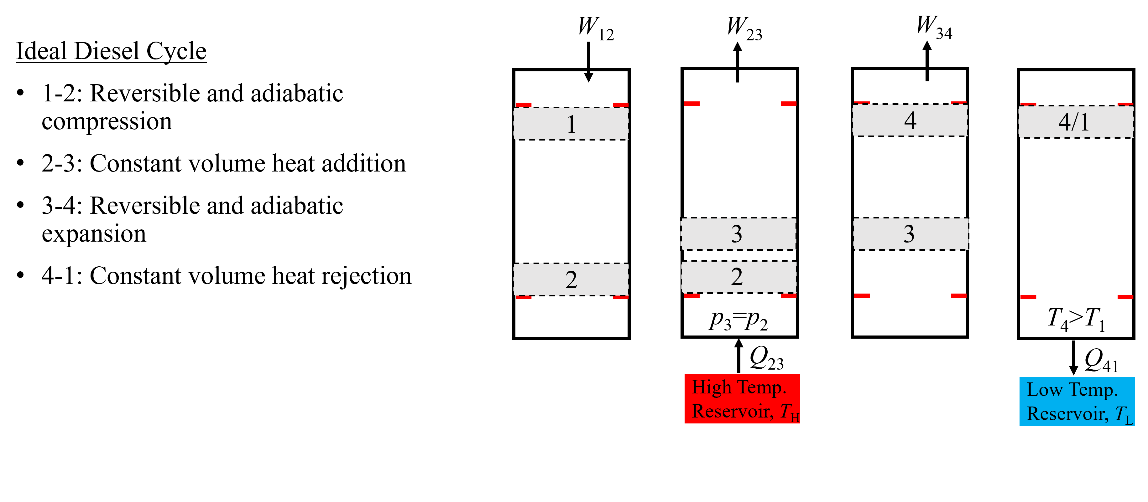
Fig. 10.9 An Ideal Diesel Cycle, composed of two piston strokes and 4 unique states.#
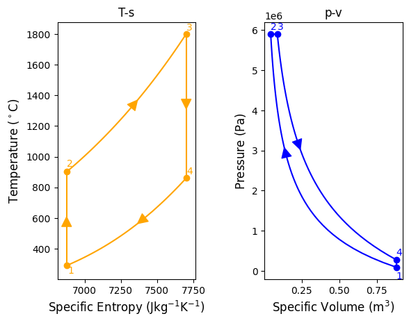
It is especially useful to visualize the Diesel Cycle using both a T-s and p-v disgram to understand where all of the work and heat transfer processes are occuring. These are shown below in Figure 10.10. Going from state 1 to state 2, notice on the T-s diagram that the isentropic work process consists of a vertical line increasing in temperature, whereas on the p-v diagram the volume decreases. As heat is added during process 2-3, temperature increases as would be expected keeping pressure constant, and notice on the p-v diagram this results in a horizontal line corresponding to an increase in volume, and thus expansion work. Expansion during process 3-4 is isentropic, corresponding to a vertical line decreasing in temperature as seen on the T-s diagram and increase in volume and corresponding decrease in pressure as seen on the p-v diagram. Finally, as heat is rejected, both temperature and entropy decrease, as well as pressure.
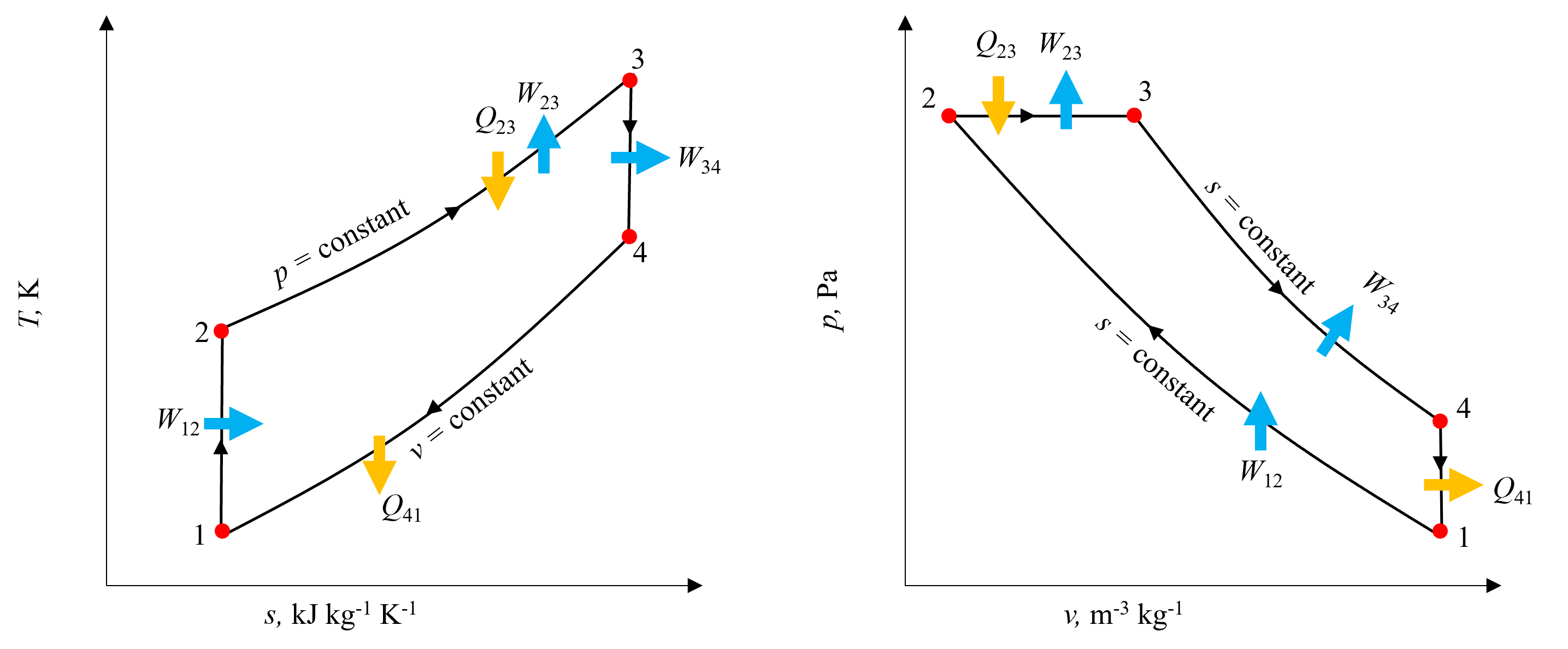
Fig. 10.10 T-s and p-v diagrams for the Ideal Diesel Cycle, indicating all relevent heat transfer and work terms, as well as isentropic and isobaric processes.#
Analysis of each of the processes within the Diesel cycle may be performed in a similar manner to the Otto Cycle. I.e., using the closed system energy conservation equation (Section 5.2 Energy Transfer and The First Law), ideal gas law (Section 4.2 Ideal Gas Equation of State), and when applicable the isentropic ideal gas equations from (Section 9.2 Isentropic Processes of Ideal Gases). The only process that is analyzed differently is process 2-3 because there are combined heat transfer and work terms. The boundary work term is straightforward to determine becuase it is assumed to occur at constant pressure, thus \(W = p\Delta V\). Starting from the closed system energy conservation equation (\(\Delta U = 0 = Q_{\rm net} - W_{\rm net}\)) for each process, the following equations can be derived.
Process 2-3: \(\Delta U_{\rm 2-3} = Q_{\rm 2-3} - W_{\rm 2-3}\)
where \(W_{\rm 2-3} = p\Delta V = p(V_{\rm 3} - V_{\rm 2}) = pm(v_{\rm 3} - v_{\rm 2})\)
thus \(Q_{\rm 2-3} = (U_{\rm 3} - U_{\rm 2}) + p(V_{\rm 3} - V_{\rm 2}) = (H_{\rm 3} - H_{\rm 2}) = mc_{\rm p}(T_{\rm 3} - T_{\rm 2})\)
As seen, the heat transfer, because it occurs at constant pressure, is equal to the change in enthalpy during process 2-3.
Like the Otto Cycle, we can use any of the isentropic equations:\(\frac{T_2}{T_1} = (\frac{v_1}{v_2})^{k-1}\), \(\frac{T_2}{T_1} = (\frac{p_2}{p_1})^{\frac{k-1}{k}}\), or \(\frac{p_2}{p_1} = (\frac{v_1}{v_2})^{k}\) for the isentropic compression and expansion processes. Another strategy would be to use Cantera to determine specific entropy at a known state condition, and equate this to the specific entropy at the state either before/after compression/expansion to determine relevent state properties. This would be useful is gas ideality or air-standard assumptions were not used.
Also like the Otto Cycle, the ideal gas law can be applied for all processes. But also relevent state properties could be solved directly using Cantera without having to assume gas ideality.
The thermal efficiency of the Ideal Diesel Cycle can be determined using (10.12) below once the appropriate heat transfer and work terms are solved for. The general startegy for this is similar to the Otto Cycle - i.e., use combinations of the above equations and/or Cantera to determine the relevent state properties. Notice the additional work term in the numerator.
10.3.2.1. Example - Analysis of an Ideal Diesel Cycle#
A diesel cycle has a compression ratio of 20:1 with an inlet at 95kPa, 290K and with volume of 0.5L. The maximum temperature is 1800K. Find the maximum pressure, net specific work and η. Assume air-standard properties.
Solution Like it is for the Otto Cycle, the compression ratio is the ratio of the largest volume relative to the minimum. We also know the most information prior to the compression process so it will likely be most useful beginning our analysis there and then working around the cycle to determine other state properties. Since process 1-2 is isentropic we can begin with an isentropic equation to determine relevent information following compression.
import cantera as ct

#determine specific heat ratio
state1 = ct.Solution('gri30.yaml')
state1.X = 'N2:0.79 O2: 0.21'
T1 = 290 #K
p1 = 95*10**3 # Pa
state1.TP = T1,p1
cp=state1.cp
cv=state1.cv
k = cp/cv
print("cv is", round(cv,2), "kJ kg-1 K-1 and k is", round(k,2))

#then we can use T2/T1 = (v1/v2)^{k-1} to solve for T2

comp_ratio = 20 #(v1/v2)
T2 = T1*(comp_ratio)**(k-1)
print("T2 after compression is", round(T2,2), "K")
cv is 720.84 kJ kg-1 K-1 and k is 1.4
T2 after compression is 960.61 K
At this point we can solve for p2 using either of the other two isentropic equations.
p2 = p1*(comp_ratio)**(k)
print("p2 after compression is", round(p2/1000,2), "kPa. This is the highest pressure in the cycle.")
p2 after compression is 6293.64 kPa. This is the highest pressure in the cycle.
Knowing this we can equate this pressure to p3 because the heat addition occurs at constant pressure. Also, the highest temperature occurs after heat addition, at state 3, so we know two state properties at state 3. We can solve for v3 knowing p3 and T3.
R_bar = 8.314 #kJ/kmol/K
M = 28.99 # kg/kmol
p3=p2 #constant pressure heat addition
T3 = 1800 #K provided in problem statement as maximum cycle temperature
v3 = (R_bar/M*T3)/(p3/1000) #m3/kg
print("v3 after combustion is", round(v3,2), "m3 kg-1")
v3 after combustion is 0.08 m3 kg-1
Knowing that the final expansion process is isentropic, we also know the specific entropy at state 3, and can equate this to specific entropy at state 4. But we don’t know any other state properties at state 4. However, we also know that v4 = v1 and we know two state properties at state 1 and can therefore determine v4.
#use ideal gas law to determine v1/v4
R_bar = 8.314 #kJ/kmol/K
M = 28.99 # kg/kmol
v1=(R_bar/M*T1)/(p1/1000) #kg
v4=v1
print("v1 and v4 are", round(v1,2), "m3 kg-1")
v1 and v4 are 0.88 m3 kg-1
We can use an isentropic equation to solve for T4.
T4 = T3*(v3/v4)**(k-1)
print("T4 after expansion is", round(T4,2), "K")
T4 after expansion is 698.49 K
The net work output can be determined by summing either the work terms or the heat transfer terms. We also need the mass, which can be determined from the given volume at state 1. Summing the work terms we get the following:
V1 = 0.5 #L
V1 = V1*.001 # to get m3
m=p1/1000*V1/(R_bar/M*T1) #kg

#Wnet = W12+W23+W34
#v1/v2 = comp_ratio

v2 = v1/comp_ratio
wnet = cv*(T1-T2)+p2*(v3-v2)+cv*(T3-T4) #J/kg/K need to divide by 1000 to get kJ
wnet=wnet/1000
Wnet = m*wnet
print("Wnet is", round(Wnet,2), "kJ")
Wnet is 0.31 kJ
Q23 = m*cp*(T3-T2)/1000
print (Q23)
eta = Wnet/Q23*100 #definition of thermal efficiency
print("The thermal efficiency is", round(eta,2), "%")
0.4837295142031297
The thermal efficiency is 65.1 %
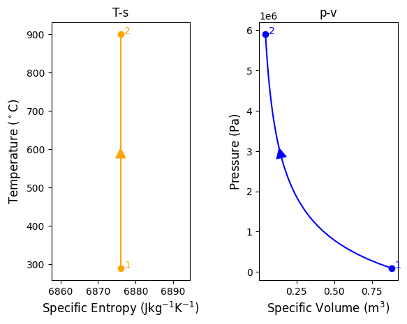
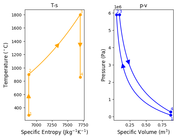
10.3.2.2. Programming Example - Plotting “Analysis of an Ideal Diesel Cycle”#
Plot the temperature versus specific entropy and pressure versus specific volume for the prior mentioned Diesel Cycle. Use Cantera rather than assuming air-standard properties. “A diesel cycle has a compression ratio of 20:1 with an inlet at 95kPa, 290K. The maximum temperature is 1800K.”
Solution We will use Cantera rather than ideal gas law and use Cantera to determine specific entropies for isentropic processes rather than using isentropic equations. We will need to generate plots ranging from extreme values at each state, and can use functions and lists to help us. But first, we should find the T, s, p and v at each state to determine our bounds. Starting with state 1.
import cantera as ct

#state1
state1 = ct.Solution('gri30.yaml')
state1.X = 'N2:0.79 O2: 0.21'
T1 = 290 #K
p1 = 95*10**3 # Pa
state1.TP = T1,p1
s1=state1.SP[0]
v1 = state1.SV[1]

print("T1 = ", round(T1,2), "K,", "s1 = ", round(s1,2), "J kg-1 K-1,", "p1 = ", round(p1,2), "Pa,", "v1 = ", round(v1,2), "m3 kg-1" )
T1 = 290 K, s1 = 6876.03 J kg-1 K-1, p1 = 95000 Pa, v1 = 0.88 m3 kg-1
#state 2
state2 = ct.Solution('gri30.yaml')
state2.X = 'N2:0.79 O2: 0.21'
comp_ratio = 20
s2=s1
v2=v1/comp_ratio
state2.SV = s2,v2
p2=state2.SP[1]
T2 = state2.TP[0]

print("T2 = ", round(T2,2), "K,", "s2 = ", round(s2,2), "J kg-1 K-1,", "p2 = ", round(p2,2), "Pa,", "v2 = ", round(v2,2), "m3 kg-1" )
T2 = 900.64 K, s2 = 6876.03 J kg-1 K-1, p2 = 5900719.94 Pa, v2 = 0.04 m3 kg-1
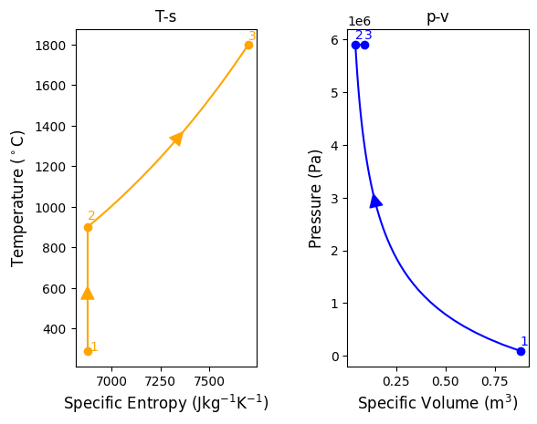
#state 3
state3 = ct.Solution('gri30.yaml')
state3.X = 'N2:0.79 O2: 0.21'
p3=p2
T3 = 1800 #K
state3.TP = T3,p3
s3=state3.SP[0]
v3 = state3.SV[1]

print("T3 = ", round(T3,2), "K,", "s3 = ", round(s3,2), "J kg-1 K-1,", "p3 = ", round(p3,2), "Pa,", "v3 = ", round(v3,2), "m3 kg-1" )
T3 = 1800 K, s3 = 7701.0 J kg-1 K-1, p3 = 5900719.94 Pa, v3 = 0.09 m3 kg-1
#state 4
state4 = ct.Solution('gri30.yaml')
state4.X = 'N2:0.79 O2: 0.21'
s4=s3
v4 = v1
state4.SV = s4,v4
T4=state4.TP[0]
p4 = state4.TP[1]

print("T4 = ", round(T4,2), "K,", "s4 = ", round(s4,2), "J kg-1 K-1,", "p4 = ", round(p4,2), "Pa,", "v4 = ", round(v4,2), "m3 kg-1" )
T4 = 860.28 K, s4 = 7701.0 J kg-1 K-1, p4 = 281816.92 Pa, v4 = 0.88 m3 kg-1
#process 1-2
import numpy as np
from scipy.optimize import minimize
import matplotlib.pyplot as plt
import matplotlib.patches as mpatches
import warnings
warnings.filterwarnings('ignore')
warnings.simplefilter('ignore')

temps_12 = np.arange(T1,T2+(T2-T1)/50,(T2-T1)/50) #50 steps between T1 and T2
# because entropy is constant, we just need a list of entropies with the same length
entropies_12= np.full(
  shape=len(temps_12),
  fill_value=s1
)
pres_12 = np.arange(p1,p2+(p2-p1)/50,(p2-p1)/50) #50 steps between p1 and p2
index = np.arange(0,len(pres_12),1)
#now we need to use Cantera to determine specific volumes for each of these pressure values
def vol(i):
    state12 = ct.Solution('gri30.yaml')
    state12.X = 'N2:0.79 O2: 0.21'
    T = temps_12[i] #K
    s = entropies_12[i]
    vguess = v1
    def solve(v):
        v=v[0]
        state12.SV = s,v # needed because there is no ST option to set state in Cantera. We will have to solve for v iterively knowing the T and P
        Tsolve = state12.TP[0]
        return abs(Tsolve-T)
    bnds = [(v2,v1)]
    res = minimize(solve, vguess, method='SLSQP',bounds=bnds)
    return res.x[0]
vols_12=[]
for i in range(len(pres_12)):
    vols_12.append(vol(i))


fig=plt.figure()
ax1= fig.add_subplot(1,2,1) # add one subplot
ax2= fig.add_subplot(1,2,2) # add a second subplot

ax1.plot(entropies_12,temps_12,color='orange')
ax2.plot(vols_12,pres_12,color='blue')

ax1.scatter(entropies_12[0],temps_12[0],color='orange')
ax1.scatter(entropies_12[-1],temps_12[-1],color='orange')
ax2.scatter(vols_12[0],pres_12[0],color='blue')
ax2.scatter(vols_12[-1],pres_12[-1],color='blue')

x1_tail = entropies_12[0]
y1_tail = temps_12[25]
x1_head = x1_tail
y1_head = temps_12[26]
arrow1 = mpatches.FancyArrowPatch((x1_tail, y1_tail), (x1_head, y1_head),
                                 mutation_scale=20,color='orange')
ax1.add_patch(arrow1)

x2_tail = vols_12[25]
y2_tail = pres_12[25]
x2_head = vols_12[26]
y2_head = pres_12[26]
arrow2 = mpatches.FancyArrowPatch((x2_tail, y2_tail), (x2_head, y2_head),
                                 mutation_scale=20,color='blue')
ax2.add_patch(arrow2)

ax1.text(entropies_12[0]+1,temps_12[0], "1", color='orange')
ax1.text(entropies_12[-1]+1,temps_12[-1], "2", color='orange')
ax2.text(vols_12[0]+.02,pres_12[0], "1", color='blue')
ax2.text(vols_12[-1]+.02,pres_12[-1], "2", color='blue')

ax1.set_xlabel('Specific Entropy $({\\mathrm{J kg^{-1}K^{-1}})}$',  fontsize=12)
ax2.set_xlabel('Specific Volume $(\\mathrm{m^{3}})$',  fontsize=12)

ax1.set_ylabel('Temperature $(\\mathrm{^\\circ C})$',  fontsize=12)
ax2.set_ylabel('Pressure $(\\mathrm{Pa})$',  fontsize=12)
#ax1.set_ylabel('$c_{\\mathrm{p}}$ $({\\mathrm{kJ kg^{-1}K^{-1}})}$',  fontsize=12)
plt.subplots_adjust(wspace=0.5) # add spacing between subplots
ax1.set_title('T-s')
ax2.set_title('p-v')

plt.savefig('Figures/diesel_cantera_12.png')# used to save the figure if you desire
plt.show()
#process 2-3
import numpy as np
from scipy.optimize import minimize
import matplotlib.pyplot as plt
import matplotlib.patches as mpatches
import warnings
warnings.filterwarnings('ignore')
warnings.simplefilter('ignore')

temps_23 = np.arange(T2,T3+(T3-T2)/50,(T3-T2)/50) #50 steps between T2 and T3
# because pressure is constant, we can make a list of pressures with the same length
pres_23= np.full(
  shape=len(temps_23),
  fill_value=p2
)
#now we need to use Cantera to determine specific volumes and entropies for each temperature and pressure value
def solve_states(i):
    state23 = ct.Solution('gri30.yaml')
    state23.X = 'N2:0.79 O2: 0.21'
    state23.TP = i,p2
    return state23.SV

entropies_23=[]
vols_23=[]
for i in temps_23:
    entropies_23.append(solve_states(i)[0])
    vols_23.append(solve_states(i)[1])

fig=plt.figure()
ax1= fig.add_subplot(1,2,1) # add one subplot
ax2= fig.add_subplot(1,2,2) # add a second subplot

ax1.plot(entropies_12,temps_12,color='orange')
ax1.plot(entropies_23,temps_23,color='orange')
ax2.plot(vols_12,pres_12,color='blue')
ax2.plot(vols_23,pres_23,color='blue')

ax1.scatter(entropies_12[0],temps_12[0],color='orange')
ax1.scatter(entropies_12[-1],temps_12[-1],color='orange')
ax1.scatter(entropies_23[-1],temps_23[-1],color='orange')
ax2.scatter(vols_12[0],pres_12[0],color='blue')
ax2.scatter(vols_12[-1],pres_12[-1],color='blue')
ax2.scatter(vols_23[-1],pres_23[-1],color='blue')

x1_tail = entropies_12[0]
y1_tail = temps_12[25]
x1_head = x1_tail
y1_head = temps_12[26]
arrow1 = mpatches.FancyArrowPatch((x1_tail, y1_tail), (x1_head, y1_head),
                                 mutation_scale=20,color='orange')
ax1.add_patch(arrow1)

x1_tail = entropies_23[25]
y1_tail = temps_23[25]
x1_head = entropies_23[26]
y1_head = temps_23[26]
arrow1 = mpatches.FancyArrowPatch((x1_tail, y1_tail), (x1_head, y1_head),
                                 mutation_scale=20,color='orange')
ax1.add_patch(arrow1)

x2_tail = vols_12[25]
y2_tail = pres_12[25]
x2_head = vols_12[26]
y2_head = pres_12[26]
arrow2 = mpatches.FancyArrowPatch((x2_tail, y2_tail), (x2_head, y2_head),
                                 mutation_scale=20,color='blue')
ax2.add_patch(arrow2)


ax1.text(entropies_12[0]+10,temps_12[0], "1", color='orange')
ax1.text(entropies_12[-1]+2,temps_12[-1]+35, "2", color='orange')
ax1.text(entropies_23[-1]+2,temps_23[-1]+25, "3", color='orange')
ax2.text(vols_12[0],pres_12[0]+.1e6, "1", color='blue')
ax2.text(vols_12[-1],pres_12[-1]+.1e6, "2", color='blue')
ax2.text(vols_23[-1],pres_23[-1]+.1e6, "3", color='blue')

ax1.set_xlabel('Specific Entropy $({\\mathrm{J kg^{-1}K^{-1}})}$',  fontsize=12)
ax2.set_xlabel('Specific Volume $(\\mathrm{m^{3}})$',  fontsize=12)

ax1.set_ylabel('Temperature $(\\mathrm{^\\circ C})$',  fontsize=12)
ax2.set_ylabel('Pressure $(\\mathrm{Pa})$',  fontsize=12)
#ax1.set_ylabel('$c_{\\mathrm{p}}$ $({\\mathrm{kJ kg^{-1}K^{-1}})}$',  fontsize=12)
plt.subplots_adjust(wspace=0.5) # add spacing between subplots
ax1.set_title('T-s')
ax2.set_title('p-v')

plt.savefig('Figures/diesel_cantera_123.png')# used to save the figure if you desire
plt.show()
#process 3-4
import numpy as np
from scipy.optimize import minimize
import matplotlib.pyplot as plt
import matplotlib.patches as mpatches
import warnings
warnings.filterwarnings('ignore')
warnings.simplefilter('ignore')

temps_34 = np.arange(T3,T4+(T4-T3)/50,(T4-T3)/50) #50 steps between T3 and T4
# because entropy is constant, we just need a list of entropies with the same length
entropies_34= np.full(
  shape=len(temps_34),
  fill_value=s3
)
pres_34 = np.arange(p3,p4+(p4-p3)/50,(p4-p3)/50) #50 steps between p3 and p4
#now we need to use Cantera to determine specific volumes for each of these pressure values
def vol(i):
    state34 = ct.Solution('gri30.yaml')
    state34.X = 'N2:0.79 O2: 0.21'
    T = temps_34[i] #K
    s = entropies_34[i]
    vguess = v3
    def solve(v):
        v=v[0]
        state34.SV = s,v # needed because there is no ST option to set state in Cantera. We will have to solve for v iterively knowing the T and P
        Tsolve = state34.TP[0]
        return abs(Tsolve-T)
    bnds = [(v3,v4)]
    res = minimize(solve, vguess, method='SLSQP',bounds=bnds)
    return res.x[0]
vols_34=[]
for i in range(len(pres_34)):
    vols_34.append(vol(i))

fig=plt.figure()
ax1= fig.add_subplot(1,2,1) # add one subplot
ax2= fig.add_subplot(1,2,2) # add a second subplot

ax1.plot(entropies_12,temps_12,color='orange')
ax1.plot(entropies_23,temps_23,color='orange')
ax1.plot(entropies_34,temps_34,color='orange')
ax2.plot(vols_12,pres_12,color='blue')
ax2.plot(vols_23,pres_23,color='blue')
ax2.plot(vols_34,pres_34,color='blue')

ax1.scatter(entropies_12[0],temps_12[0],color='orange')
ax1.scatter(entropies_12[-1],temps_12[-1],color='orange')
ax1.scatter(entropies_23[-1],temps_23[-1],color='orange')
ax1.scatter(entropies_34[-1],temps_34[-1],color='orange')
ax2.scatter(vols_12[0],pres_12[0],color='blue')
ax2.scatter(vols_12[-1],pres_12[-1],color='blue')
ax2.scatter(vols_23[-1],pres_23[-1],color='blue')
ax2.scatter(vols_34[-1],pres_34[-1],color='blue')

x1_tail = entropies_12[0]
y1_tail = temps_12[25]
x1_head = x1_tail
y1_head = temps_12[26]
arrow1 = mpatches.FancyArrowPatch((x1_tail, y1_tail), (x1_head, y1_head),
                                 mutation_scale=20,color='orange')
ax1.add_patch(arrow1)

x1_tail = entropies_23[25]
y1_tail = temps_23[25]
x1_head = entropies_23[26]
y1_head = temps_23[26]
arrow1 = mpatches.FancyArrowPatch((x1_tail, y1_tail), (x1_head, y1_head),
                                 mutation_scale=20,color='orange')
ax1.add_patch(arrow1)

x1_tail = entropies_34[0]
y1_tail = temps_34[25]
x1_head = x1_tail
y1_head = temps_34[26]
arrow1 = mpatches.FancyArrowPatch((x1_tail, y1_tail), (x1_head, y1_head),
                                 mutation_scale=20,color='orange')
ax1.add_patch(arrow1)

x2_tail = vols_12[25]
y2_tail = pres_12[25]
x2_head = vols_12[26]
y2_head = pres_12[26]
arrow2 = mpatches.FancyArrowPatch((x2_tail, y2_tail), (x2_head, y2_head),
                                 mutation_scale=20,color='blue')
ax2.add_patch(arrow2)

x2_tail = vols_34[25]
y2_tail = pres_34[25]
x2_head = vols_34[26]
y2_head = pres_34[26]
arrow2 = mpatches.FancyArrowPatch((x2_tail, y2_tail), (x2_head, y2_head),
                                 mutation_scale=20,color='blue')
ax2.add_patch(arrow2)

ax1.text(entropies_12[0]+10,temps_12[0], "1", color='orange')
ax1.text(entropies_12[-1]+2,temps_12[-1]+35, "2", color='orange')
ax1.text(entropies_23[-1]+2,temps_23[-1]+25, "3", color='orange')
ax1.text(entropies_34[-1]+2,temps_34[-1]+25, "4", color='orange')
ax2.text(vols_12[0],pres_12[0]-.3e6, "1", color='blue')
ax2.text(vols_12[-1],pres_12[-1]+.1e6, "2", color='blue')
ax2.text(vols_23[-1],pres_23[-1]+.1e6, "3", color='blue')
ax2.text(vols_34[-1],pres_34[-1]+.1e6, "4", color='blue')

ax1.set_xlabel('Specific Entropy $({\\mathrm{J kg^{-1}K^{-1}})}$',  fontsize=12)
ax2.set_xlabel('Specific Volume $(\\mathrm{m^{3}})$',  fontsize=12)

ax1.set_ylabel('Temperature $(\\mathrm{^\\circ C})$',  fontsize=12)
ax2.set_ylabel('Pressure $(\\mathrm{Pa})$',  fontsize=12)
#ax1.set_ylabel('$c_{\\mathrm{p}}$ $({\\mathrm{kJ kg^{-1}K^{-1}})}$',  fontsize=12)
plt.subplots_adjust(wspace=0.5) # add spacing between subplots
ax1.set_title('T-s')
ax2.set_title('p-v')

plt.savefig('Figures/diesel_cantera_1234.png')# used to save the figure if you desire
plt.show()
#process 4-1
import numpy as np
from scipy.optimize import minimize
import matplotlib.pyplot as plt
import matplotlib.patches as mpatches
import warnings
warnings.filterwarnings('ignore')
warnings.simplefilter('ignore')

temps_41 = np.arange(T4,T1+(T1-T4)/50,(T1-T4)/50) #50 steps between T3 and T4
# because volume is constant, we can make a list of specific volumes with the same length
vols_41= np.full(
  shape=len(temps_41),
  fill_value=v4
)

pres_41 = np.arange(p4,p1+2*(p1-p4)/50,(p1-p4)/50) #50 steps between p1 and p2

#now we need to use Cantera to determine specific entropy for each of these temperature pressure pairs
def entropy(i):
    state41 = ct.Solution('gri30.yaml')
    state41.X = 'N2:0.79 O2: 0.21'
    T = temps_41[i] #K
    v = vols_41[i]
    sguess = s4
    def solve(s):
        s=s[0]
        state41.SV = s,v # needed because there is no ST option to set state in Cantera. We will have to solve for s iterively knowing the T and v
        Tsolve = state41.TP[0]
        return abs(Tsolve-T)
    bnds = [(s1,s4)]
    res = minimize(solve, sguess, method='SLSQP',bounds=bnds)
    return res.x[0]
entropies_41=[]
for i in range(len(temps_41)):
    entropies_41.append(entropy(i))

fig=plt.figure()
ax1= fig.add_subplot(1,2,1) # add one subplot
ax2= fig.add_subplot(1,2,2) # add a second subplot

ax1.plot(entropies_12,temps_12,color='orange')
ax1.plot(entropies_23,temps_23,color='orange')
ax1.plot(entropies_34,temps_34,color='orange')
ax1.plot(entropies_41,temps_41,color='orange')
ax2.plot(vols_12,pres_12,color='blue')
ax2.plot(vols_23,pres_23,color='blue')
ax2.plot(vols_34,pres_34,color='blue')
ax2.plot(vols_41,pres_41,color='blue')

ax1.scatter(entropies_12[0],temps_12[0],color='orange')
ax1.scatter(entropies_12[-1],temps_12[-1],color='orange')
ax1.scatter(entropies_23[-1],temps_23[-1],color='orange')
ax1.scatter(entropies_34[-1],temps_34[-1],color='orange')
ax2.scatter(vols_12[0],pres_12[0],color='blue')
ax2.scatter(vols_12[-1],pres_12[-1],color='blue')
ax2.scatter(vols_23[-1],pres_23[-1],color='blue')
ax2.scatter(vols_34[-1],pres_34[-1],color='blue')

x1_tail = entropies_12[0]
y1_tail = temps_12[25]
x1_head = x1_tail
y1_head = temps_12[26]
arrow1 = mpatches.FancyArrowPatch((x1_tail, y1_tail), (x1_head, y1_head),
                                 mutation_scale=20,color='orange')
ax1.add_patch(arrow1)

x1_tail = entropies_23[25]
y1_tail = temps_23[25]
x1_head = entropies_23[26]
y1_head = temps_23[26]
arrow1 = mpatches.FancyArrowPatch((x1_tail, y1_tail), (x1_head, y1_head),
                                 mutation_scale=20,color='orange')
ax1.add_patch(arrow1)

x1_tail = entropies_34[0]
y1_tail = temps_34[25]
x1_head = x1_tail
y1_head = temps_34[26]
arrow1 = mpatches.FancyArrowPatch((x1_tail, y1_tail), (x1_head, y1_head),
                                 mutation_scale=20,color='orange')
ax1.add_patch(arrow1)

x1_tail = entropies_41[25]
y1_tail = temps_41[25]
x1_head = entropies_41[26]
y1_head = temps_41[26]
arrow1 = mpatches.FancyArrowPatch((x1_tail, y1_tail), (x1_head, y1_head),
                                 mutation_scale=20,color='orange')
ax1.add_patch(arrow1)

x2_tail = vols_12[25]
y2_tail = pres_12[25]
x2_head = vols_12[26]
y2_head = pres_12[26]
arrow2 = mpatches.FancyArrowPatch((x2_tail, y2_tail), (x2_head, y2_head),
                                 mutation_scale=20,color='blue')
ax2.add_patch(arrow2)

x2_tail = vols_34[25]
y2_tail = pres_34[25]
x2_head = vols_34[26]
y2_head = pres_34[26]
arrow2 = mpatches.FancyArrowPatch((x2_tail, y2_tail), (x2_head, y2_head),
                                 mutation_scale=20,color='blue')
ax2.add_patch(arrow2)

ax1.text(entropies_12[0]+10,temps_12[0]-50, "1", color='orange')
ax1.text(entropies_12[-1]+2,temps_12[-1]+35, "2", color='orange')
ax1.text(entropies_23[-1]+2,temps_23[-1]+25, "3", color='orange')
ax1.text(entropies_34[-1]+2,temps_34[-1]+25, "4", color='orange')
ax2.text(vols_12[0],pres_12[0]-.3e6, "1", color='blue')
ax2.text(vols_12[-1],pres_12[-1]+.1e6, "2", color='blue')
ax2.text(vols_23[-1],pres_23[-1]+.1e6, "3", color='blue')
ax2.text(vols_34[-1],pres_34[-1]+.1e6, "4", color='blue')

ax1.set_xlabel('Specific Entropy $({\\mathrm{J kg^{-1}K^{-1}})}$',  fontsize=12)
ax2.set_xlabel('Specific Volume $(\\mathrm{m^{3}})$',  fontsize=12)

ax1.set_ylabel('Temperature $(\\mathrm{^\\circ C})$',  fontsize=12)
ax2.set_ylabel('Pressure $(\\mathrm{Pa})$',  fontsize=12)
#ax1.set_ylabel('$c_{\\mathrm{p}}$ $({\\mathrm{kJ kg^{-1}K^{-1}})}$',  fontsize=12)
plt.subplots_adjust(wspace=0.5) # add spacing between subplots
ax1.set_title('T-s')
ax2.set_title('p-v')

plt.savefig('Figures/diesel_cantera_1234.png')# used to save the figure if you desire
plt.show()
10.3.3. Stirling Cycle#
The Stirling Cycle is based on a reciprocating dual piston-cylinder design that recuperates heat internally to improve efficiency. The internal heat recuperation is acheived using a regenerator, which is a type of thermal storage medium that receieves and transfers heat to different processes within the cycle. In contrast to the Otto and Diesel cycles, the Stirling Engine is heated via an external source and is therfore sometimes referred to as an external combustion engine - but in reality the heat source can be of any type, renewable or fossil. Because they rely on external heat transfer, these heat engines are often of interest for renewable energy systems that have a source of high temperature heat such as concentrated solar energy. In fact, in 2008, Sandia National Laboratories and Stirling Energy Systems set a world record 31.25% conversion efficiency of solar energy to electrical work using a Stirling engine coupled with a solar parabolic dish (https://newsreleases.sandia.gov/sandia-stirling-energy-systems-set-new-world-record-for-solar-to-grid-conversion-efficiency/). Since that time, photovoltaic efficiencies have surpassed this value and can be as high as 46.7% when coupled with solar concentration (https://www.nrel.gov/pv/cell-efficiency). Nevertheless, Stirling heat engines remain of interest for a variety of applications due to their high efficiencies and flexibility to be integrated with varying heat sources.
The purpose of the regenerator is similar to the regenerator discussed prior for the Brayton cycle. That is, the temperature following expansion is well above the ambient temperature and in principle can be transferred internally prior to heat addition. The benefit is reduced external heat input to acheive the same final state, and external heat addition at the highest temperature possible. However, a Stirling Cycle, which is based on recipricating piston-cylinders cannot simply recuperate heat from a hot stream and transfer it to a cooler stream with the help of a heat exchanger operating at steady state conditions. Rather, because of the cyclical nature of the engine, the heat must be stored in a regenerator and transferred back for later use. To enable this, the Stirling Engine operates with two pistons, one hot and one cooler, with the hot piston transferring energy to the regenerator. The regenerator, in principle is any type of porous solid with a large specific heat that stores the internal heat and it is assumed that the heat stored in the working gas is negligable compared to the solid. The mechanics of the Stirling cycle are complex and cannot easily be broken down into discrete processes as easily as the Otto and Diesel cycles. Therefore, our analysis is limited to the highly idealized Stirling cycle which consist of four fully reversible processes. Using air-standard assumptions, the Ideal Stirling Cycle can be summarized as:
Constant temperature heat addition and expansion
Constant volume internal heat transfer to a regenerator
Constant temperature heat rejection and compression
Constant volume internal heat transfer from a regenerator
The idealized Stirling Cycle is shown below in Figure 10.11. Starting on the left process 1-2 consists of heat transfer from a high temperature reservoir and expansion of the hot side at a constant temperture. Then, process 2-3 consists of internal heat transfer to the regenerator while the total system volume remains constant. Notice that the volume of the hot side decreases while the cold side increases - but the net work associated with these processes is negligable and not considered in our analysis. Following internal heat transfer to the regenerator, the cold side is compressed while heat is simultanesouly transferred to the low temperature reservoir. Finally, during process 4-1, the regenerator transfers heat to the hot side, prior to external heating and to restart the cycle.
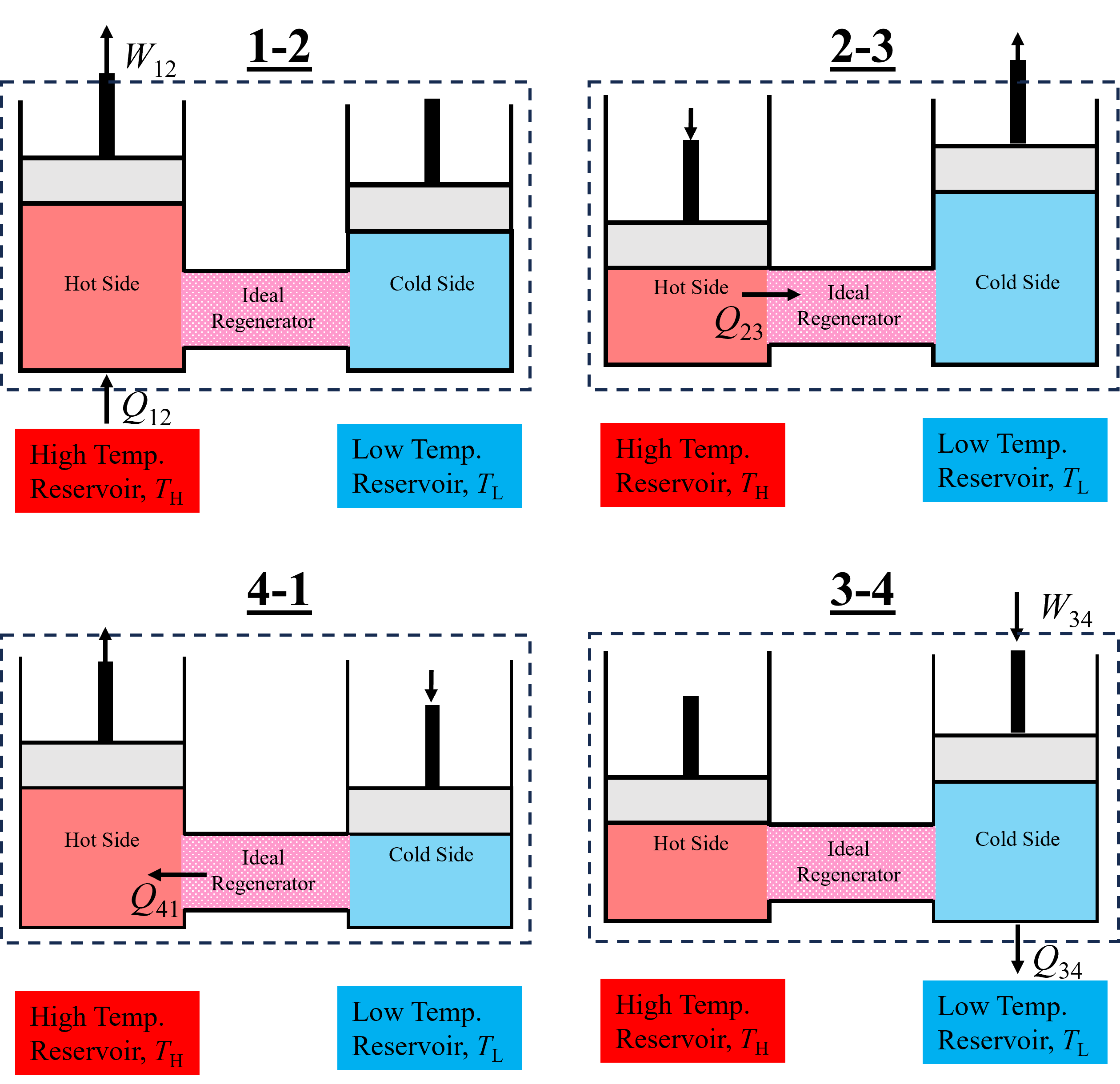
Fig. 10.11 An Ideal Stirling Cycle, composed of two pistons designed to recuperate heat internally with the help of a regenerator.#
The Ideal Stirling Cycle is presented on a T-s a diagram below in Figure 10.12. Notice that there are no longer any isentropic processes like there were for the Otto, Diesel, Brayton and Carnot cycles. However, because each process in the cycle and completly reversible, the maximum efficiency that can be acheived is, in principle, the Carnot Efficiency.
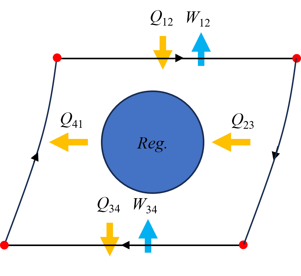
Fig. 10.12 T-s diagram for the Ideal Stirling Cycle. Notice that compared to the Carnot Cycle, there are no isentropic processes, but the external heat addition terms occur at constant temperature.#
Analysis of each of the processes within the Stirling cycle may be performed in a similar manner to the prior piston-cyclinder based cycles, with two notable exceptions. First, because there are no isentropic processes the isentropic ideal gas equations from Section 9.2 Isentropic Processes of Ideal Gases cannot be used. Second, because the compression and expansion process occur isothermally and reversibly, we can use the appropriate polytopic work equations with n = 1 from Section 6.2 More on Boundary Work - Polytropic Process. Thus, to analyze each process only the closed system energy conservation equation (Section 5.2 Energy Transfer and The First Law), ideal gas law (Section 4.2 Ideal Gas Equation of State) and Section 6.2 More on Boundary Work - Polytropic Process equations are necessary.
The polytopic work for an isothermal process (i.e. n = 1) may be evaluated using the equations below for expansion and compression, respectively.
In addition to calculating efficiency like the prior gas power cycles, the Stirling Cycle efficiency may also be calculated using the Carnot Efficiency equation, shown below in (10.16).
10.3.3.1. Example - Analysis of an Ideal Stirling Cycle#
Consider an ideal Stirling cycle. At the beginning of the isothermal compression process, air is at 100 KPa and 300K. Total heat supplied from a source at 1700K is 800 kJ/kg. Determine the pressure after expansion, the net specific work and thermal efficiency, η. Assume air-standard properties.
Solution We will start at state 3, prior to compression where we know the most information. We will use ideal gas law but below is a comparison to using Cantera as well.
import cantera as ct

#state3

R_bar = 8.314 #kJ/kmol/K
M = 28.99 # kg/kmol

state3 = ct.Solution('gri30.yaml')
state3.X = 'N2:0.79 O2: 0.21'
T3 = 300 #K
T4 = T3 #process 3-4 is isothermal
p3 = 100*10**3 # Pa
state3.TP = T3,p3
v3_cantera = state3.SV[1] #specific volume calculated using Cantera
v3 = (R_bar/M*T3)/(p3/1000) #m3 kg-1
v2=v3 # process 2-3 is constant volume

print("v3 calculated using Cantera is = ", round(v3_cantera,2), "m3 kg-1")
print("v3 calculated using ideal gas law  is = ", round(v3,2), "m3 kg-1")
v3 calculated using Cantera is =  0.86 m3 kg-1
v3 calculated using ideal gas law  is =  0.86 m3 kg-1
Solution Now we will use the additional information provided.
T1 = 1700 #K
T2 = T1 #isothermal for process 1-2
q12 = 800 #kJ/kg

w12=q12 # apply first law, delta_U = 0 because constant temperature

R_bar = 8.314 #kJ/kmol/K
M = 28.99 # kg/kmol

#Recognize we know two properties at state 2.
p2 = (R_bar/M*T2)/(v2) #kPa

print("The specific heat transfer and work to and by the cycle is = ", round(q12,2), "kJ kg-1")
print("p2 calculated using ideal gas law is is = ", round(p2,2), "kPa")
The specific heat transfer and work to and by the cycle is =  800 kJ kg-1
p2 calculated using ideal gas law is is =  566.67 kPa
Solution Now we know the specific expansion work, p2, v2 and we can solve for v1 using (10.12)
# w12 = p2v2ln(v2/v1)
import numpy as np
v1 = v2/np.exp(w12/p2/v2)
v4=v1
print("v1 calculated using polytropic work equation is = ", round(v1,2), "m3 kg-1")
v1 calculated using polytropic work equation is = 0.17 m3 kg-1
Solution We now know two state properties at 4 and can calulate p4
R_bar = 8.314 #kJ/kmol/K
M = 28.99 # kg/kmol

#Recognize we know two properties at state 4.
p4 = (R_bar/M*T4)/(v4) #kPa
print("p4 calculated using ideal gas law is is = ", round(p4,2), "kPa")
p4 calculated using ideal gas law is is = 515.98 kPa
Solution Knowing, v4, v3 p3/p4 we can solve for w34 using (10.13)
# w12 = p3v3ln(v4/v3)
import numpy as np
w34 = p3/1000*v3*np.log(v4/v3)
q34 = w12 # first law for an isothermal process
print("The specific heat transfer and work from and to the cycle is = ", round(w34,2), "kJ kg-1")
The specific heat transfer and work from and to the cycle is = -141.18 kJ kg-1
w_net = w12+w34
eta = w_net/q12 * 100

print("The pressure after expansion is ", round(p2,2), "kPa")
print("The net specific work is ", round(wnet,2), "kJ kg-1" )
print("The thermal efficiency, η, is ", round(eta,2) , "%")
The pressure after expansion is  566.67 kPa
The net specific work is  551.34 kJ kg-1
The thermal efficiency, η, is  82.35 %
Solution Let’s compare our computed efficiency to the Carnot Efficiency
Th = T1
Tl = T3
eta_carnot = (1-Tl/Th) * 100

print("The Carnot efficiency, η, is ", round(eta_carnot,2) , "%")
The Carnot efficiency, η, is 82.35 %
10.3.4. Ericsson Cycle#
The is another type of regenerative gas power cycle that enables constant temperature heat addition and heat rejection. It is composed of 4 completely reversible processes, so the theoretical thermal efficiency is also equivilent of the Carnot efficiency, like the Stirling cycle. Unlike the Stirling cycle, the Ericsson Cycle is based on a steady flow system that utilizes turbines and compressors that are coupled with heat addition and heat rejection, respectively. Thus, expansion and compression are also not isentropic. The major distinction in terms of analysis compared to the Stirling cycle is that the regeneration occurs via a heat exchanger (i.e. no sensible energy storage), and the heat transfer during regeneration occurs at constant pressure, just like the regenerator in the Brayton Cycle.
Using air-standard assumptions, the four full reversible processes of the Ideal Ericsson Cycle can be summarized as:
Constant temperature heat addition and expansion
Constant pressure internal heat transfer to a regenerator
Constant temperature heat rejection and compression
Constant pressure internal heat transfer from a regenerator
Becuase the Ericsson Cycle is composed of steady state devices, each process should be analyzed using the steady state open system energy balance discussed in Section 7 First Law of Thermodynamics - Open Systems. Like all other gas power cycles, the ideal gas law can be applied to any state within the cycle, and like the Stirling Cycle isentropic ideal gas equations from Section 9.2 Isentropic Processes of Ideal Gases cannot be used. Unlike the Stirling Cycle, the work terms associated with compression and expansion should be evaluated using the Section 9.3 Reversible Steady State Workequation when k = 1 (i.e. isothermal), shown below,
10.3.5. Exercise 8#
A stationary gas-turbine power plant operates on a simple ideal Brayton cycle with air as the working fluid. The air enters the compressor at 95 kPa and 290 K and the turbine at 760 kPa and 1100 K. Heat is transferred to air at a rate of 35,000 kW. Determine the power delivered by this plant (a) assuming constant specific heats at room temperature and (b) accounting for the variation of specific heats with temperature.
A gas turbine power plant operates on the simple Brayton cycle with air as the working fluid and delivers 32 MW of power. The minimum and maximum temperatures in the cycle are 310 and 900 K, and the pressure of air at the compressor exit is 8 times the value at the compressor inlet. Assuming an isentropic efficiency of 80% for the compressor and 86% for the turbine, determine the mass flow rate of air through the cycle. Account for the variation of specific heats with temperature.
A Brayton cycle using air as the working fluid operates at steady state with intercooling and reheating. The net power output is 10 MW. Use data provided below:
Sketch the T-s diagram for the cycle
Determine the mass flowrate of air, in kg/s
The rate of heat transfer, in kW, during all heat addition stages
The thermal efficiency
State |
p (kPa) |
T (K) |
h (kJ/kg) |
|---|---|---|---|
1 |
100 |
300 |
300.19 |
2 |
300 |
410.1 |
411.22 |
3 |
300 |
300 |
300.19 |
4 |
1200 |
444.8 |
446.50 |
5 |
1200 |
1111 |
1173.84 |
6 |
1200 |
1450 |
1575.57 |
7 |
300 |
1034.3 |
1085.31 |
8 |
300 |
1450 |
1575.57 |
9 |
100 |
1111 |
1173.84 |
10 |
100 |
444.8 |
446.50 |
Consider an ideal gas-turbine cycle with two stages of compression and two stages of expansion. The pressure ratio across each stage of the compressor and turbine is 3. The air enters each stage of the compressor at 300 K and each stage of the turbine at 1200 K. Determine the thermal efficiency of the cycle, assuming (a) no regenerator is used and (b) a regenerator with 75 percent effectiveness is used. Use variable specific heats.
Air at ambient conditions is compressed with a compression ratio of r = 12 in an ideal Otto cycle. 700 kJ/kg of is added during the constant volume process.
What is the net specific work (wnet) of the cycle?
What is the thermal efficiency (nth,otto) of this process?
What is the thermal efficiency (nth) not assuming constant specific heats?
An ideal Otto cycle has a compresion ratio of 10. The air is at P = 120 kPa and T = 300 K before compression and reaches P = 4.5 MPa and T = 1500 K after heat addition.
What is the specific heat addition (q) to the system?
What is the thermal efficiency of the cycle?
An ideal Diesel cycle has a cutoff ratio of 3 and a compression ratio of 16. The air is at ambient conditions prior to compression.
What is the heat addition (q) to the system?
What is the thermal efficiency of the cycle?
Air in an ideal diesel cycle is at P = 4 MPa and T = 1500 K after constant pressure heat addition. The cutoff ratio is 1.7 and the compression ration is 18.
What is the heat addition (q) to the system?
What is the net specific work (wnet) in the cycle?
What is the thermal efficiency (nth) of the cycle?
A power plant uses an ideal brayton cycle with a pressure ratio of 10. The gas enters the compressor at ambient conditions and enters the turbine at T 1500 K.
What is the heat addition to the system?
What is the thermal efficiency of the cycle?
If the net power is P = 1 MJ, what is the mass flowrate (m)?
Section 12.8 Exercise 8 Solutions
test