3. Brief Introduction to Thermodynamics: Systems , Processes, States and Properties

3.1. Thermodynamic Systems

Thermodynamics is a broad field of study that is concerned with systems undergoing processes from one state to another. A system is very generally defined as anything we want to study that contains a quantity of matter, for example a gas turbine, chemical reactor, boiler, photovoltaic panel, ourselves, a house, commercial building or even our planet earth. Everything external to the system is considered the surroundings. The system is distinguished from its surroundings by its boundary. A system is characterized by its properties, where properties are macroscopically averaged physical characteristics such as temperature ($T$), mass ($m$), volume ($V$) and pressure ($p$), or perhaps less familiar viscosity ($\mu$), thermal conductivity ($k$), and heat capacity ($c_{\mathrm{p}}$ or $c_{\mathrm{v}}$). In the classical view of thermodynamics, we are concerned only with systems large enough such that properties are measureable. Thus, the classical, or macroscopic, view of thermodynamics is not concerned events occuring at the molecular level. Events occuring at the molecular level, when averaged over a large number of molecules, describes the macroscopic behavior and this is typically modeled through statistical means since the number of molecules required to describe macroscopic behavior is very large and computaitonally intensive.

When the properties of a system change, its state changes and the system is said to undergo a process. The path that the process takes, for example the pressure dependency as volume changes, are important when evaluating heat ($Q$) or work ($W$) interactions, as their magnitude depends on the path that was taken to go from one state to another. Therefore, heat and work are referred to as path functions. For example, we will show in later chapters that mechanical work ($W_{\mathrm{m}\mathrm{e}\mathrm{c}\mathrm{h}}$) = $\int pdV$, and thus evaluation of $W_{\mathrm{m}\mathrm{e}\mathrm{c}\mathrm{h}}$ depends on the functional dependence, or path of $p$ on $V$ (i.e., $p=f(V)$).

State functions on the other hand, such as volume, do not depend on the path but only the initial and final states. That is, $\mathrm{\Delta }V=\int dV$. As such, path functions in differential form are inexact differentials and state functions are exact differentials. We distinguish between inexact and exact differentials with the symbols $\delta$ and $d$, respectively, for example $\delta W_{\mathrm{m}\mathrm{e}\mathrm{c}\mathrm{h}}$ and $dV$.

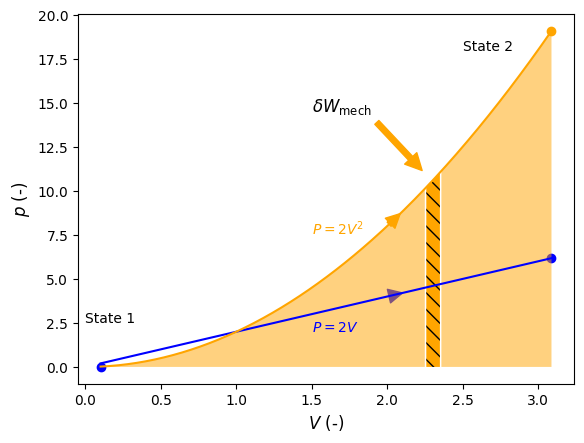
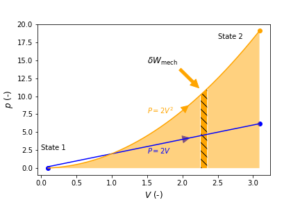
Consider Figure 3.1 below that shows $p$ verses $V$ for two hypotetical processes. The orange curve represents a path going from $V_1=1$ at State 1 to $V_2=3$ at State 2, where $p=2V^2$, and the blue curve represents a path going from $V_1=1$ at State 1 to $V_2=3$ at State 2, where $p=2V$. $\mathrm{\Delta }V$ for both processes is equal to 2 and is independent of the path. $W_{\mathrm{m}\mathrm{e}\mathrm{c}\mathrm{h}}$ however, which equals $\int pdV$, is represented by the area under its curve, or the path, as indicated by the light shaded orange area in the case of the first process. A differential amount of mechanical work, $\delta W_{\mathrm{m}\mathrm{e}\mathrm{c}\mathrm{h}}$, is indicated by the hashed orange area.

Click to show

import numpy as np
import matplotlib.patches as mpatches
import matplotlib.pyplot as plt
import warnings
warnings.filterwarnings('ignore')
warnings.simplefilter('ignore')
x_tail = 2
y_tail = 2*2**2
y_tail2 = 2*2
x_head = 2.1
x_head2 = 2.12
y_head = 2*2.1**2
y_head2 = 2*2.12
#dx = x_head - x_tail
#dy = y_head - y_tail

fig,ax= plt.subplots(1,1)
vol=np.arange(0.1,3.1,0.01)
ax.plot(vol,2*vol,color='blue')
ax.plot(vol,2*vol**2,color='orange')
ax.scatter(vol[0],2*vol[0]**2,color='blue')
ax.scatter(vol[-1],2*vol[-1]**2,color='orange')
ax.scatter(vol[-1],2*vol[-1], color='blue')

arrow1 = mpatches.FancyArrowPatch((x_tail, y_tail), (x_head, y_head),
                                 mutation_scale=20,color='orange')
arrow2 = mpatches.FancyArrowPatch((x_tail, y_tail2), (x_head2, y_head2),
                                 mutation_scale=20,color='blue')
ax.add_patch(arrow1)
ax.add_patch(arrow2)
#ax.text(0,2.5, "State 1", fontname="Arial")
ax.text(0,2.5, "State 1")
ax.text(2.5,18, "State 2")
ax.text(1.5,7.5, "$P=2V^2$",color='orange')
ax.text(1.5,2, "$P=2V$",color='blue')
ax.set_xlabel('$V$ (-)', fontsize=12)
ax.set_ylabel('$p$ (-)', fontsize=12)
ax.annotate('$\delta W_{\mathrm{mech}}$', (2.25,11), (1.5,14.5), arrowprops=dict(color='orange', shrink=0.05), fontsize=12)
ax.fill_between(vol,2*vol**2, where= (vol >= 2.25) & (vol <= 2.35),facecolor = "orange",hatch='\\\\')
ax.fill_between(vol,2*vol**2, where= (vol >= 2.35) ,facecolor = "orange", alpha=0.5)
ax.fill_between(vol,2*vol**2, where= (vol <= 2.25) ,facecolor = "orange", alpha=0.5)
#plt.xlabel('$V$ (-)')
#plt.ylabel('$P$ (-)')
plt.savefig('Figures/pv_work.png')# used to save the figure if you desire
plt.show()

Fig. 3.1 Pressure verses volume for two different procecess going from State 1 to State 2. The work associated with each process is indicated by the areas under each curve. A exemplary amount of differential work is indicated by the dashed region.

Thermodynamic processes are all bound by the First and Second Laws of Thermodynamics [von Baeyer, 1998]. The First Law of Thermodynamics traces it’s roots back to Count Rumford’s experiments in the 18th century while boring a cannon [Thompson, 1798]. He showed that the production of heat was essentially inexastiable, as long as mechanical work was applied to the cannon by rotating a cannon borer. This led to Count Rumford’s claim that “heat is work”, from which the name thermodynamics was born. When coupled with James Prescott Joules more precise measurements that quantified the equivilency of heat and work, the First Law of Thermodynamics was conceived, which at its core states that energy is always conserved, and when it is destroyed in one form, it reappears as another [Joule, 1850]. The Second Law of Thermodynamics is more subtle than the first, and puts contraints on the directionality of processes [Ness, 1969]. For example, we know that mechanical work is readily transformed to thermal energy, such as when a paddle wheel does work to a system it will heat up. However, the reverse scenario, converting heat to mechanical work, does not happen spontaneously - i.e., if we heat up a system it will not necessarily cause a paddle wheel to rotate, even though we have not violated the First Law. The Second Law says that if heat is to be converted to mechanical work, then not all of it is available, and some will have to be rejected from the system at a lower temperature [Borgnakke and Sonntag, 2017]. This is the basis of a heat engine. The fraction of the heat that is not converted to work is intimately tied to the temperature at which the heat is delivered, and thus the second law also gives a quality to energy. That is, energy at a higher temperature has a greater capacity to do work than at a lower temperature, leading to higher efficiency. The second law also puts constraints on the direction of energy transfer, and says that heat will always flow from hot to cool in the absense of any other effects. The microscopic view nicely explains things such as the second law of thermodyanmics, and the limited directionality of processes [Dill and Bromberg, 2011]. We will touch on microscopic aspects of thermodynamics in this book in later chapters, but the focus is on the macroscopic view.

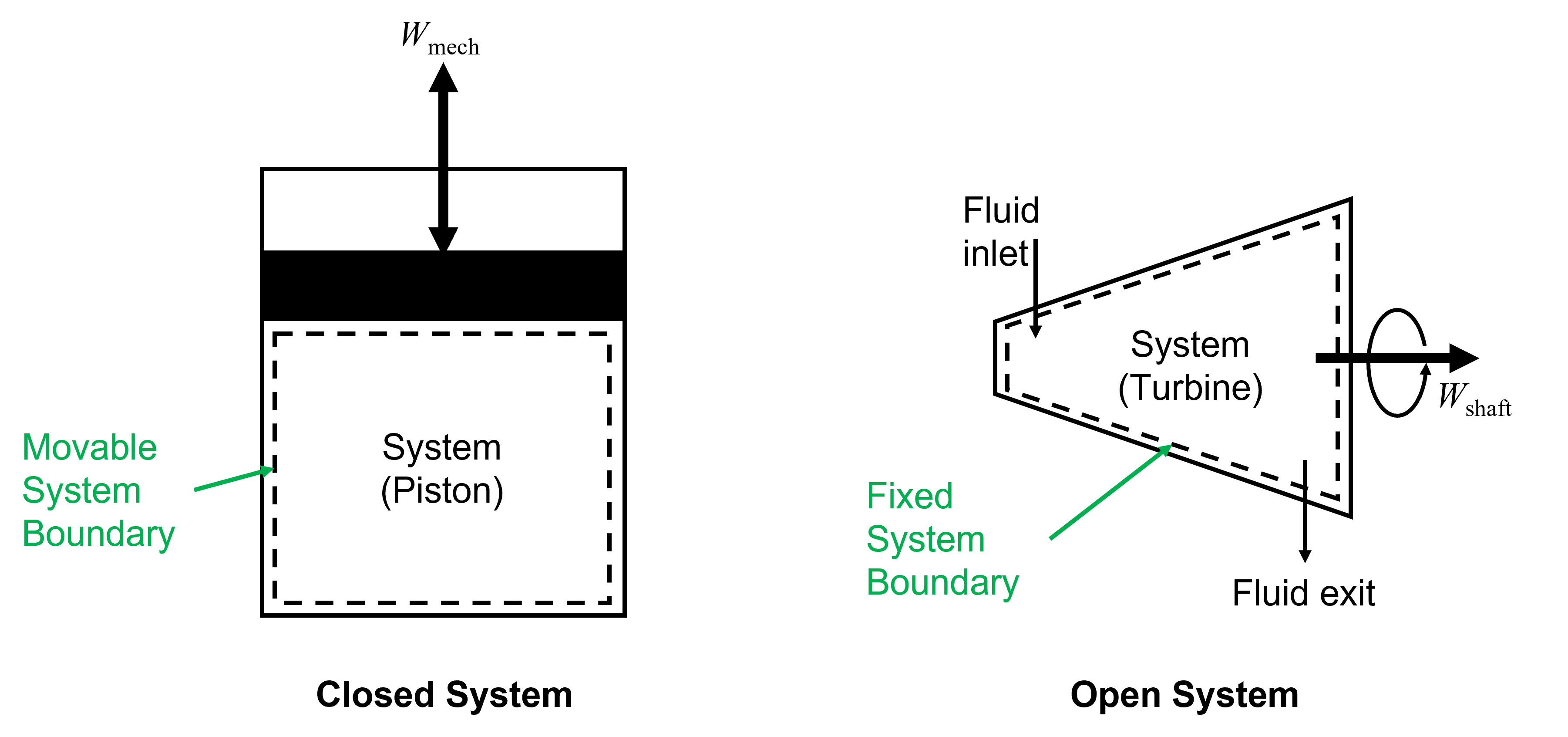
As mentioned, the system can be anything we wish to study and it is distinguised form its surroundings by its boundary. The system boundary can be fixed or moving, real or imaginary. For example, a piston-cylinder as shown below in Figure 3.2 on the left has a moving boundary that expands and contracts as the piston moves. A gas turbine, also shown in Figure 3.2 on the right which has an inlet and exit for a working fluid to enter and leave has imaginary boundaries drawn around these points and real boundaries elsewhere, and the entire system boundary is fixed.

Thermodynamic systems can be categorized one of two ways, either as a closed system (or control mass) or an open system (or control volume). As the names imply, a closed system always contains a fixed quantity of matter, but energy may flow into and out of the system. An open system is one in which energy and matter may flow into and out of the system. The only way energy may be transferred to or from a system is through heat ($Q$) or work ($W$) interactions, which we will expand on later when we formally introduce the First Law of Thermodynamics and the concept of Energy Conservation. Because the mass is fixed in the case of the piston-cylinder, but mechanical work ($W_{\mathrm{m}\mathrm{e}\mathrm{c}\mathrm{h}}$) can be done to or by the system (i.e. energy is transferred), or heat can be transferred to or from it, it is considered a closed system. In the case of the turbine, matter enters and exits and there is also energy transfer in the form of shaft work ($W_{\mathrm{s}\mathrm{h}\mathrm{a}\mathrm{f}\mathrm{t}}$), and thus this is considered an open system.

Fig. 3.2 Left) A piston-cylinder shcematic which is exemplary of a closed system with a moving boundary. As the piston moves up or down in the cylinder the system boundary also moves accordingly. Right) A turbine schematic, which is an open system with a fixed system boundary.The turbine produces shaft work as a result of gases entering at high pressure and high temperature, expanding across turbine blades causing the shaft to rotate, and then exiting at reduced temperature and pressure.

3.2. Properties and Processes

A thermodynamic system is at equilibrium when none of its properties are changing with time. There are several types of equilibrium, including thermal, mechanical, phase and chemical, and a system is not in thermodynamic equilibrium unless all equilibrium types are satisfied. For many processes a particular property will remain constant, indicated by the prefix, iso. For example, processes at constant temperature are referred to as isothermal, constant pressure as isobaric, constant volume as isochoric (or isometric), and constant entropy (a property that will be discussed in later sections) as isentropic.

Properties can be placed into two general categories, namely extensive or intensive. A property is extensive if its value for an overall system is dependent on the sum of its parts, for example volume ($V$), mass ($m$) or energy ($E$). Intensive properties are those which have a value that is independent on the size of the system, for example temperature ($T$) or density ($\rho$). Density is defined as the ratio of mass divided by volume, or:

(3.1)$$\begin{gathered} \begin{array}{r}\mathrm{d}\mathrm{e}\mathrm{n}\mathrm{s}\mathrm{i}\mathrm{t}\mathrm{y}(\rho )=\underset{V\to V^{\prime } \\ }{lim}\frac{m}{V}\end{array} \end{gathered}$$

where $V^{\prime }$ is the smallest volume for which a definite value exists. When extensive properties are normalized per unit mass they are referred to as specific (or mass specific) properties and indicated with a lower case character (e.g., $e=\frac{E}{m}$). They thus become intensive properties. The reciprocal of density is specific volume ($v$) with SI units $\frac{{\mathrm{m}}^3}{\mathrm{k}\mathrm{g}}$.

(3.2)$$\begin{gathered} \begin{array}{r}\text{specific volume}(v)=\underset{V\to V^{\prime } \\ }{lim}\frac{V}{m}=\frac{1}{\rho }\end{array} \end{gathered}$$

When extensive properties are normalized per unit mole they are referred to as molar specific properties and indicated with a lower case character with an overhead bar. They thus also become intensive properties. For example, molar specific volume ($\overline{v}$) has SI units $\frac{{\mathrm{m}}^3}{\mathrm{k}\mathrm{m}\mathrm{o}\mathrm{l}}$. Molar specific properties are related to their mass specific counterparts by multiplying the molecular weight ($M$) of the substance by the mass specific property:

(3.3)$$\overline{v}=vM$$

which we can readily see from observation of the units, or unit analysis. I.e., $\frac{{\mathrm{m}}^3}{\mathrm{k}\mathrm{m}\mathrm{o}\mathrm{l}}=\frac{{\mathrm{m}}^3}{\mathrm{k}\mathrm{g}}\frac{\mathrm{k}\mathrm{g}}{\mathrm{k}\mathrm{m}\mathrm{o}\mathrm{l}}$

3.3. Units and Dimensional Homogeneity

SI units and prefixes will be used consitently throughout this textbook and a good understanding of unit analysis, or dimensional homogenity is critial for success, as seen in the simple example above. Primary and secondary SI units, as well as common SI prefixes are shown below in Table 3.1.

Table 3.1 :SI Units and Prefixes

Primary SI Units	Secondary SI Units	SI Prefixes
mass (m) - kg	force (F) - N ($\frac{\mathrm{k}\mathrm{g}\mathrm{m}}{{\mathrm{s}}^2}$)	${10}^{12}$ - tera, T
length (l) - m	pressure (p) - Pa ($\frac{\mathrm{N}}{{\mathrm{m}}^2}$)	${10}^9$ - giga, G
time (t) - s	energy (E) - J ($\mathrm{N}\mathrm{m}$)	${10}^6$ - mega, M
temperature (T) - K	power (P) - W ($\frac{\mathrm{J}}{\mathrm{s}}$)	${10}^3$ - kilo, k
amount of matter (n) - mol	—	${10}^{-3}$ - milli, m

A typical unit for electrical energy is kWh, which can be related to the SI unit for energy, J, on the basis of understanding dimensional homogeneity. For example,

$1\mathrm{k}\mathrm{W}\mathrm{h}=1\frac{\mathrm{k}\mathrm{J}}{\mathrm{s}}\mathrm{h}=1\frac{\mathrm{k}\mathrm{J}}{\mathrm{s}}\frac{3600\mathrm{s}}{\mathrm{h}}=3600\mathrm{k}\mathrm{J}$

There are many where cases you can infer the solution to a problem only by analyzing the units, without understanding what all of the properties mean. More complex examples are shown below.

3.3.1. Example

The specific heat of water is roughly 4.2 $\frac{\mathrm{k}\mathrm{J}}{\mathrm{k}\mathrm{g}°\mathrm{C}}$ and its density is 1 $\frac{\mathrm{g}}{\mathrm{m}\mathrm{L}}$. How much energy, in kJ, is required to heat 10 gallons of water to 50 °C? (Note: there are roughly 3.8 L per gallon)

#Solution:
# 10 gallons * 3.8 L/gallon * 1000 mL/1L * 1g/mL * 1kg/1000 g * 4.2kJ/kg°C * 50°C
ans=str((10*3.8*1000*4.2*50)/1000)
print(ans +" kJ")

7980.0 kJ

3.3.2. Example

The average electric utility rate in Gainesville, FL is $\frac{\mathrm{\$}0.10}{\mathrm{k}\mathrm{W}\mathrm{h}}$. If your electric bill per month, on average, is $150 determine your total electrical energy consumption over the course of a year, in GJ.

#Solution:
# $150/month * 1kWh/$0.10 * 1000Wh/1kWh * 3600J/1Wh * 1GJ/10^9J * 12months/1yr
ans=str((150*1000*3600*12)/(.1*10**9))
print(ans +" GJ/year")

64.8 GJ/year

3.3.3. Example

Imagine you installed a solar panel on your home that produces power 8 hours per day with a rated power of 5 kW. The lifetime of the panels is 30 years and they cost $10,000 to install. Will these panels save you money over this time period?

#Solution:
#Energy Produced by Solar Panels/Year: 5kW (wattage) * 8hr/day * 365days/year 
energyprod=(5*8*365)
#Cost savings/year: energy produced/year * average electric utility rate: 14600 kWh/year * $0.10/kWh
savings=(energyprod*0.1)
print("Energy produced by panels/year: " + str(energyprod) + " kWh/year")
print("Cost savings/year: $" + str(savings) +"/year" )
#Cost savings over 30 year period: cost savings/year * 30 years - initial investment of $10,000
totalsavings= str(savings*30 -10000)
print("Total savings amounts to: $" + totalsavings)
print("Therefore, the solar panel will save you money over a 30 year period.")

Energy produced by panels/year: 14600 kWh/year
Cost savings/year: $1460.0/year
Total savings amounts to: $33800.0
Therefore, the solar panel will save you money over a 30 year period.

3.4. Temperature and the Zeroth Law of Thermodynamics

Temperature ($T$) is an intensive thermodynamic property related to the kinetic energy of molecules in a system. In fact, it is an indicator of the internal energy (which is introduced later in Section 5 First Law of Thermodynamics - Introduction to Closed Systems) of a system and has important implications for the directionality of processes - i.e. heat will flow spontaneously from hot to cold systems in the absense of an adiabatic barrier, until thermal equilibrium between the systems is reached, or the point at which their temperatures are identical. The Zeroth Law of Thermodynamics says that when two objects are in thermal equilibrium with a third object, that they are in thermal equilibrium with each other. The third object is usually a thermometer. The Zeroth Law states that the quantity that is the same for two systems in thermal equilibrium with each other is temperature, and thus this essentially defines temperature. Although this may seem intuitive, it actually forms the basis of the first and second laws, but was discovered afterwards, thus the name Zeroth.

The thermodynamic temperature scale in SI units is the Kelvin ($K$) scale, where the lowest temperature is absolute zero (i.e., the point at which the molecules in the system have zero kinetic energy). This is related to the Celsius scale by the following relationship.

(3.4)$$T(\mathrm{K})=\mathrm{T}(°\mathrm{C})+273.15$$

Thus, whenever we are interested in changes in temperature, we can use either the Kelvin or Celsius scale and will arrive at equivilent answers. Although differences in temperature will be common to see throughout calculations in this book, we will usually err on the side of safety and convert to the Kelvin scale for problems in this textbook. The Celsius scale is related to the Fahrenheit scale by the following relationship.

(3.5)$$T(°\mathrm{F})=1.8\mathrm{T}(°\mathrm{C})+32$$

The Fahrenheit scale is related to the thermodynamic temperature scale in the English unit system, Rankine ($R$).

(3.6)$$T(\mathrm{R})=\mathrm{T}(°\mathrm{F})+459.67$$

(3.7)$$T(\mathrm{R})=1.8\mathrm{T}(\mathrm{K})$$

3.5. Pressure

Pressure ($P$) is an intensive property that is, by definition, a normal force exerted by a fluid per unit area, or:

(3.8)$$\begin{gathered} \begin{array}{r}\text{pressure}(P)=\underset{A\to A^{\prime } \\ }{lim}\frac{F_{normal}}{A}\end{array} \end{gathered}$$

where A` is the smallest measurable area for which a definitive value exists. SI unites for pressure are Pascal (Pa), where 1 Pa = 1 $\frac{\mathrm{N}}{{\mathrm{m}}^2}$. More commonly, kPa or MPa are used simply because atmospheric pressure, which is 100 kPa, is large when expressed in Pa. It is also common to see SI units bar.

1 bar = 10⁵ Pa = 0.1 MPa = 100 kPa.

Atmospheric units are also common to see and related to SI units by the following.

1 atm = 1.01325 bar

The English unit pounds per square inch, or psi, is also a common unit of pressure but not used often in this textbook.

1 atm = 14.696 psi, where psi = $\frac{\mathrm{l}\mathrm{b}\mathrm{f}}{\mathrm{i}{\mathrm{n}}^2}$

Finally, mmHg or Torr, is another common pressure unit and is related to atmospheric pressure by the following

1 atm = 760 mmHg (or Torr)

Pressure is usually represented either as absolute or Gage Absolute pressure is measured with repect to absolute valcuum and gage pressure with respect to the surrounding pressure. For the most part, absolute pressure will be used throughout this textbook, unless otherwise indicated.