6. First Law of Thermodynamics - Boundary Work and Specific Heats#
In the previous chapter Section 5 First Law of Thermodynamics - Introduction to Closed Systems we learned about various forms of heat transfer and work interactions and used or evaluated these with the help of energy conservation equation for closed systems and evaluation of the relevant properties. We learned that for stationary, closed systems undergoing a process, the energy equation reduces to \(\Delta U = Q_{\rm net} - W_{\rm net}\) , where the internal energy is the combined microscopic forms of energy of the system (e.g., thermal energy), \(Q_{\rm net}\) is the net heat transfer and \(W_{\rm net}\) is the net work. When the heat transfer and work terms are added to the energy equation in numerical form, the correct sign should be applied to them, depending on the direction of the interaction. I.e., positive for heat transfer to the system and work from the system, and negative for heat transfer from the system and work to the system. Note that if you are solving for either \(Q\) or \(W\), then the resulting sign is indicitive of the direction of heat transfer and you do not need to apply the correct sign. Refer to the section Section 5.2 Energy Transfer and The First Law from chapter Section 5 First Law of Thermodynamics - Introduction to Closed Systems for more discussion.
For fixed volume systems, boundary work can be ignored, and in the absense of other work interactions the energy equation reduces to \(Q_{\rm net} = \Delta U\). However, for variable volume systems such as piston-cylinders undergoing compression/expansion, we cannot ignore the boundary work. Refer to the prior examples Section 5.2.2.4 Example - Constant Volume System and Section 5.2.2.5 Example - Constant Pressure System from chapter Section 5 First Law of Thermodynamics - Introduction to Closed Systems. For the special case of constant pressure compression/expanion, we also showed that \(Q_{\rm net} = \Delta H\), where H is the extensive property enthalpy and captures the internal energy and boundary work into a single term (\(h = u + pv\)). Refer to the section Section 5.3 Enthalpy from chapter Section 5 First Law of Thermodynamics - Introduction to Closed Systems for more discussion.
In this chapter the concept of reversible, polytropic work is introduced which allows us to readily evaluate boundary work when pressure is not constant. Further, specific heats, \(c_{\rm p}\) and \(c_{\rm v}\) are introduced, which are thermodynamic properties that enable evaluation of internal energy and enthalpy changes by measurement of other system properties, such as temperature and pressure, which are readily measurable.
6.1. More on Boundary Work - Reversible Processes#
Reversible processes are those which can occur in the forward and reverse directions without any external input from the surroundings. They are idealized processes that are not possible in nature, but provide reference for the maximum or minimum input that is required to drive a process. For example, the maximum work output acheivable by lowering a weight from a high to low elevation is the change in gravitational potential energy, or \(W = mg(h_2-h_1)\). For a reversible process, the reverse direction (i.e., raising the weight back to its original elevation) should be equally possible without any added external input from the surroundings. The only way this is possible is if the work output gained from dropping the weight were used to raise the weight back to its original height. In reality, the work output will be lower than the change in potential energy because of other external factors that render processes irreversible, such as friction. Further, more work will need to be put into raising the mass than the idealized reversible work in order to overcome the frictional losses.
As seen from the above example, friction is one type of irreversibility. Another is any form of heat transfer over a finite temperature gradient. This is because heat transfer can only occur in one direction spontaneously, i.e., from hot to cold. The only way to transfer heat back from a cool body to a warmer one would require an external work input (i.e., a heat pump, which we will learn about following a more in depth disussion of the Second Law of Thermodynamics, in later chapters), thereby rendering the process irreversible. Finally, another irreversibility is the unconstrained release of pressure, which is especially relevant for expansion and compression processes in piston-cylinder devices.
To extract the maximum work via a reversible expansion process, expansion should be constrained in such a way that the external force (and thus pressure) that the system is acting against decreases gradually as volume increases. In essence, the internal and external forces are almost equal to each other, but one is infintessimally larger or smaller than the other. You can imagine this as an infinite series of weights or stops, such that as one is removed, the volume increases infinitesimally and the pressure decreases infinitesimally. In the opposite extreme case, or one that is completely irreversible resulting in the minimum work, the pressure is released in an unconstrained manner and the external force that the system works against is a minimum. Examples of unconstrained and constrained piston expansion, and the resulting pressure-volume curve that dictates the work output, is shown in Figure 6.1 below. Starting on the left, the expansion is completly unconstrained - the weights (indicated in red) are all removed simultanesouly and the piston expands until the internal and external pressures are equilibrated. Because all of the weight is removed at once, the external force during the expansion process is a minimum the entire time (indicated by the red area), resulting in minimum work (recall \(W_{\rm mech} = \int_{1}^{2} F_{\rm ext}dx\) or \(W_{\rm mech} = \int_{1}^{2} pdV\)). The middle case is partially constrainted and the weight has been removed in two iterations. By leaving part of the mass on the piston during the first expansion, more work was done compared to the unconstrained case because the external force was greater. This can be visualized by the added green area in the pressure-volume curve. Finally, on the right is a more constrined case where the weight has been divided into several pieces and removed one at a time. In this case, even more work is done because the external pressure, or force, is greater during more of the expansion process. This can be visualized by the added blue areas in the pressure-volume curve. The idealized reversible process is shown in the dashed line, where the internal force is only infinitesimally greater than the external force, which would be described by a series of inifinite weights. Of course, to realize the reversible process it would take an infinite period of time, which is why we can only approximate reversible processes but never realize them.
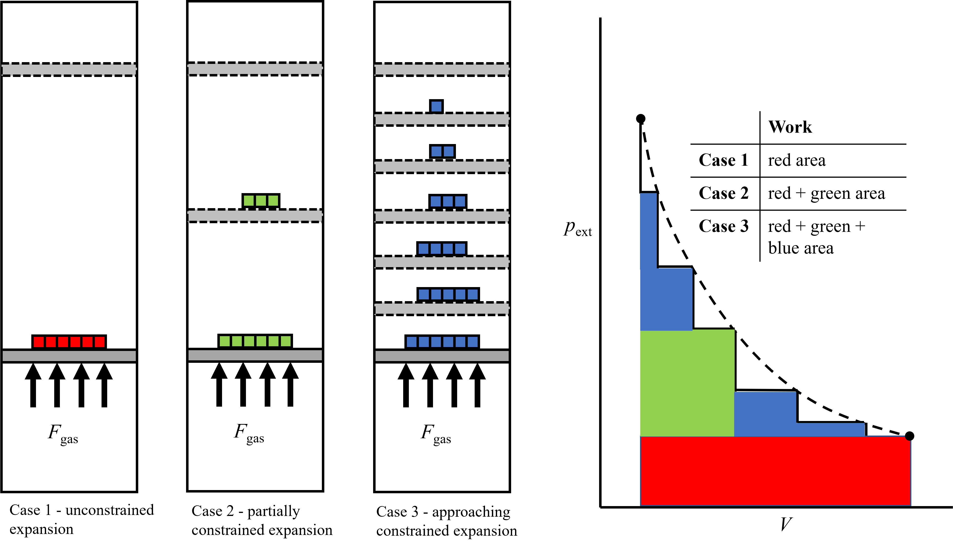
Fig. 6.1 Schematic depicting unconstrined expansion (left), partially constrained expansion (middle), and even more constrained expansion (right) which is the closest to a reversible process. The work associated with each of these processes is indicated by the magnitude of the areas under the colored portions. Red is the left unconstrined case, red and green the intermediate case and red, green and blue the most constrained case. The dashed line represents the competely constrained case, in which the internal pressure is only infinitesimally larger than the external pressure during the entire expansion process.#
6.2. More on Boundary Work - Polytropic Process#
Constant pressure expansion and compression processes were discussed in Section 5.2.2.1 Mechanical Work. In this scenario, evaluation of the boundary work from \(W_{\rm mech} = \int_{1}^{2} pdV\) is straightforward and reduces to \(W_{\rm mech} = P\Delta V\). However, there are an infinite number of paths that could be taken during compression and expansion, and often pressure is not constant during these processes, as seen during the example of reversible expansion discussed above. For the special case of reversible compression and expansion processes involving an ideal gas, these are called polytropic processes. The relationship between pressure and volume during polytropic processes is described mathematically as:
where \(n\) is a constant called the polytropic exponent. Thus, during a polytropic process the product of \(pV^{\rm n}\) remains constant, even as pressure and volume both change. This expression is true using specific volume as well, i.e., \(pv^{\rm n}\) remains constant during a process. An example of different polytropic paths are shown below in Figure 6.2.
Show code cell content
import numpy as np
import matplotlib.pyplot as plt
import numpy as np
n=np.arange(0,2,0.5)
pi,Vi = 100,.5
const = pi*Vi**n
V=np.arange(.5*Vi,2*Vi,.25*Vi)
p=[]
for i in range(len(n)):
    p.append(const[i]/(V**n[i]))
for i in range(len(n)):
    plt.plot(V,p[i])
plt.annotate('n = 0', (0.25,110), color='Blue', fontsize=12)
plt.annotate('n = .5', (0.25,145), color='Orange', fontsize=12)
plt.annotate('n = 1', (0.25,203), color='Green', fontsize=12)
plt.annotate('n = 1.5', (0.30,250), color='Red', fontsize=12)
plt.annotate('$pV^\mathrm{n} = const$', (0.5,200), color='Black', fontsize=12)
plt.xlabel('$V$ $(\mathrm{m^3})$',  fontsize=12)
plt.ylabel('$p$ $({\mathrm{kPa})}$',  fontsize=12)
plt.savefig('Figures/polytropic_exponent.png')# used to save the figure if you desire
plt.show()
<>:17: SyntaxWarning: invalid escape sequence '\m'
<>:18: SyntaxWarning: invalid escape sequence '\m'
<>:19: SyntaxWarning: invalid escape sequence '\m'
<>:17: SyntaxWarning: invalid escape sequence '\m'
<>:18: SyntaxWarning: invalid escape sequence '\m'
<>:19: SyntaxWarning: invalid escape sequence '\m'
/tmp/ipykernel_1670/3073569994.py:17: SyntaxWarning: invalid escape sequence '\m'
  plt.annotate('$pV^\mathrm{n} = const$', (0.5,200), color='Black', fontsize=12)
/tmp/ipykernel_1670/3073569994.py:18: SyntaxWarning: invalid escape sequence '\m'
  plt.xlabel('$V$ $(\mathrm{m^3})$',  fontsize=12)
/tmp/ipykernel_1670/3073569994.py:19: SyntaxWarning: invalid escape sequence '\m'
  plt.ylabel('$p$ $({\mathrm{kPa})}$',  fontsize=12)
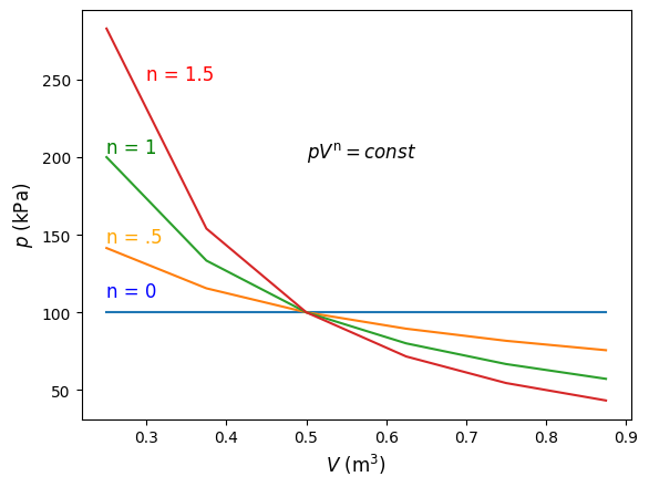
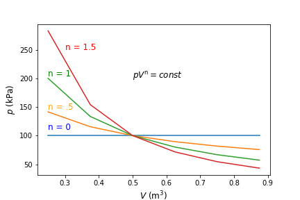
Fig. 6.2 Pressure verses volume for reversible processes with different polytropic exponents, \(n\). The polytropic exponent dictates the path that is taken and is dependent on the amount of heat transfer during the expansion/compression process.#
In the case of \({\rm n} = 0\), this is an isobaric process, or \(p_1=p_2\). When \({\rm n} = 1\), or \(p_1V_1=p_2V_2\), this is representative of an isothermal process. We can see this from analysis of the ideal gas law, where
If the process is isothermal (\(T_1=T_2\)) and in a closed system with constant mass (\(m_1=m_2\)), then equation (8.2) reduces to the same as we conclude from a polytropic process with \(\rm n=1\)
This is only possible if heat is added or rejected during expansion or compression, respectively. And as n varies, this is representative of different degrees of heat transfer during during the compression or expansion process.
6.2.1. Evaluating Polytropic Process#
Starting from the definition of mechanical work
and rearranging the polytropic equation to obtain pressure as a function of volume
we can insert this into the work equation and integrate analytically
which reduces to the following in the case where n \(\neq\) 1 and const. = \(p_1V_1^\rm n\) or \(p_2V_2^\rm n\).
In the case where n = 1, then
and with const. = \(p_1V_1\) = \(p_2V_2\).
6.2.1.1. Example - Evaluating Polytropic Work - Isothermal Process#
2 kg of N2 at 100 kPa and 15 °C is contained within a piston cylinder. It is compressed to a final pressure of 600 kPa. During compression heat is transferred from the N2 and the temperature remains constant. Determine the work input required. \(M_{\rm N2}\) = 28 kg kmol-1
Solution - Recall that if polytropic expansion or compression is conducted isothermally then n=1. Therefore, the work equation we can use is from equation (8.9). We will need to use either the ideal gas law or Cantera to solve for the specific volume at State 1 (100 kPa and 15 °C) and State 2 (600 kPa and 15 °C), and then determine the volume at each state by multiplying the specific volume times the mass. Alternatively, we could just use the ideal gas law to directly solve for the volume. Then knowing pressure and volume at states 1 and 2 we can directly solve for the work using (8.9).
import cantera as ct
#First State 1
T1,p1,m = 15, 100000, 2 # celsius, Pa, kg
species1 = ct.Nitrogen()# define species1 as nitrogen
species1.TP = 273.15+T1, p1
v1=species1.UV[1]
V1=m*v1
print(V1, "m3, Using Cantera") #units m^3
def v(p,T): # we could have also used ideal gas
    return 8.314/28*(T1+273.15)/(p1/1000) # divide p by 100 because of units for ideal gas constant in kJ
print(m*v(p1,T1), "m3, Using Ideal Gas Equation") #units m^3
1.7099180898606285 m3, Using Cantera
1.711199357142857 m3, Using Ideal Gas Equation
import cantera as ct
#State 2
T2,p2,m = 15, 600000, 2 # celsius, Pa, kg
species1 = ct.Nitrogen()# define species1 as nitrogen
species1.TP = 273.15+T1, p2
v2=species1.UV[1]
V2=m*v2
print(V2, "m3, Using Cantera") #units m^3
0.2846013748242659 m3, Using Cantera
W=p1*V1*np.log(V2/V1)
print(W, "J") #units J
print("The boundary work is", round(W/1000,2), "kJ") #units kJ
-306607.33315565734 J
The boundary work is -306.61 kJ
Notice, we could have also used only specific volumes within the logarithm and didn’t necessarily need to evaluate \(V_2\). Also notice the negatice sign, which is an indication that work was done to the system - since this was a compression process, which requires work, this makes sense.
6.2.1.2. Example - Evaluating Polytropic Work Numerically with Python’s scipy Package#
Repeat above example, but use the Python package scipy.integrate sub-package to evaluate the boundary work integral. This is a numerical integration procedure described here (https://docs.scipy.org/doc/scipy/tutorial/integrate.html)- there are also ways to perform analytical computations using the Sympy package but its use is outside the scope of this text. There is extensive documentation of you would like to learn more - https://docs.sympy.org/latest/modules/integrals/integrals.html. For now, we will leverage the scipy package and import the integrate sub-package as the following line of code \(import\) \(scipy.integrate\) \(as\) \(integrate\).
Solution - Recall that if polytropic expansion or compression is conducted isothermally then n=1. We wish we to evaluate the integral \(W_{\rm mech} = \int_{1}^{2} pdV\), where \(pV = \rm const.\) and \(p_1V_1 = \rm const.\). Therefore, we can define pressure as a function of volume, and by solving for \(V_1\) at State 1 (100 kPa and 15 °C) and \(V_2\) at State 2 (600 kPa and 15 °C) using cantera we can evaluate the integral using \(scipy.integrate\)
import cantera as ct
#State 1
T1,p1,m = 15, 100000, 2 # celsius, Pa, kg
#State 2
T2,p2,m = 15, 600000, 2 # celsius, Pa, kg
species1 = ct.Nitrogen()# define species1 as nitrogen
species1.TP = 273.15+T1, p1
v1=species1.UV[1]
V1=m*v1
species1.TP = 273.15+T2, p2
v2=species1.UV[1]
V2=m*v2
print(V1, "and", V2, "are V1 and V2 in m^3")
1.7099180898606285 and 0.2846013746854079 are V1 and V2 in m^3
def p(V):
    return p1*V1/V #express pressure as a function of volume
import scipy.integrate as integrate
work = integrate.quad(p, V1, V2) # quad is used for general purpose integration
print(work)
(-306607.3332390848, 5.80017246903583e-07)
The first value is the value of the integral and the second is the estimated error. We are interested in the value which is \(res[0]\).
print("The boundary work is", round(work[0]/1000,2), "kJ") # Units kJ. Notice the value is identical to above.
The boundary work is -306.61 kJ
6.2.1.3. Example - Evaluating Polytropic Work - Non-Isothermal Process#
2 kg of N2 at 100 kPa and 15 °C is contained within a piston cylinder. It is compressed to a final pressure of 600 kPa and temperature of 100 °C. Determine the work input required. \(M_{\rm N2}\) = 28 kg kmol-1
Solution - To determine the work, we will have to evaluate the polytopic exponent, n. We have enough information to solve for the volume at State 1 and State 1 using either Cantera or ideal gas law.
import cantera as ct
#State 1
T1,p1,m = 15, 100000, 2 # celsius, Pa, kg
species1 = ct.Nitrogen()# define species1 as nitrogen
species1.TP = 273.15+T1, p1
v1=species1.UV[1]
V1=m*v1

#State 2
T2,p2,m = 100, 600000, 2 # celsius, Pa, kg
species1 = ct.Nitrogen()# define species1 as nitrogen
species1.TP = 273.15+T2, p2
v2=species1.UV[1]
V2=m*v2
print(V1, "and", V2, "are V1 and V2 in m^3")
1.7099180898606285 and 0.3696353158332322 are V1 and V2 in m^3
Then, knowing \(p_1\), \(V_1\) and \(p_2\), \(V_2\), we can solve for n, knowing:
\(pV^{\rm n} = \rm const.\)
thus
\(p_1V_1^{\rm n} = p_2V_2^{\rm n}\)
\({\rm ln}p_1+{\rm nln}V_1 = {\rm ln}p_2+{\rm nln}V_2\)
\({\rm nln}\frac{V_1}{V_2} ={\rm ln}\frac{p_2}{p_1}\), and finally
\(n=\frac{{\rm ln}\frac{p_2}{p_1}}{{\rm ln}\frac{V_1}{V_2}}\)
n=np.log(p2/p1)/np.log(V1/V2)
print(round(n,3), "is the polytropic exponent")
1.17 is the polytropic exponent
We could also call the scipy.optimize subpackage in python to use the fsolve function to solve for n directly without algebraic simplification as seen below.
from scipy.optimize import fsolve
def poly(n):
    return p1*V1**n-p2*V2**n
res = fsolve(poly,.8)
print(round(res[0],3), "is the polytropic exponent")
1.17 is the polytropic exponent
Knowing \(p_1\), \(V_1\), \(p_2\), \(V_2\), and n we can then solve directly for the work using equation (8.7)
work = (p2*V2-p1*V1)/(1-n)
print("The boundary work is", round(work/1000,2), "kJ")
The boundary work is -299.12 kJ
6.3. Specific Heats#
Recall the energy equation in differential form, which says \(dU = \delta Q- \delta W\). While we have just learned how to quantify work, which is readily determined via evaluation of easily measureable properties (i.e., pressure and volume), it would be equaly beneficial to quantify the heat transfer from some readily measureable properties. However, if we wish to use the energy equation to help us solve for the heat transfer, internal energy, or enthalpy, are not properties that are readily measurable. Therefore, a property called specific heat is defined, which relates either internal energy and enthalpy changes to changes in temperature, which is readily measureable. The specific heat is defined as the energy required to raise the temperature of a system with mass 1 gram by 1 \(^\circ\)C (or 1 K). The amount of energy depends on if the system volume is fixed or allowed to vary (as in a piston-cylinder), and thus there are two specific heats that are definied. For a fixed volume system, the specific heat (\(c_\rm v\)) is indicated with a subscript v to indicate constant volume. For a constant pressure system, the specific heat (\(c_\rm p\)) is indicated with a subscript p to indicate constant pressure.
The difference between \(c_\rm v\) and \(c_\rm p\) is exemplified below in Figure 6.3. In the fixed volume system on the left there is no work done by the system, and the heat transfer is the change in internal energy. For the fixed pressure system on the right, there is work done because of expansion as heat is added to the system. Because of the extra work associated with raising the temperature of the fixed pressure system, the required energy change to raise its temperature by 1 K is greater than the fixed volume system.
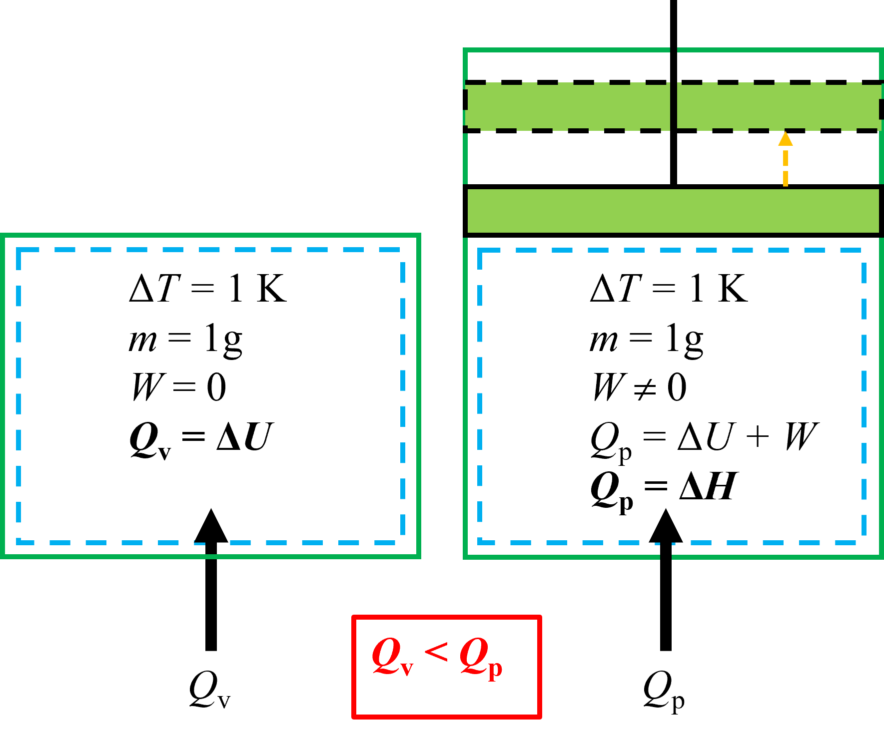
Fig. 6.3 Schematic depicting the difference between specific heat at constant volume (\(c_\rm v\)) and specific heat at constant pressure (\(c_\rm p\)). Because there is work done in the fixed pressure system on the right as energy is added, due to expansion, the required energy to raise its temperature by 1 K is greater than the fixed volume system.#
6.3.1. Specific Heat at Constant Volume#
Starting from the specific energy equation in differential form, replacing the differential work with \(pdv\),
and differentiating with respect to temperature at constant volume
The left hand side of the equation, \(\left( \frac{\partial q}{\partial T}\right)_{\rm v}\), is by definition the specific heat, \(c_\rm v\). Therefore,
6.3.2. Specific Heat at Constant Pressure#
Likewise, again starting from the specifc energy equation in differential form
and differentiating the enthalpy equation (\(h=u+pv\)) and solving for \(du\)
we can substitute this back into the energy equation to show that
And differentiating with respect to remperature, keeping pressure constant
The left hand side of the equation, \(\left( \frac{\partial q}{\partial T}\right)_{\rm p}\), is also by definition the specific heat, \(c_\rm p\). Therefore,
6.3.2.1. Molar Specific Heats#
The above equations can also be expressed on a molar basis. That is
Thus, although for the ensuing discussion where specific heats are expressed only on a mass basis, corresponding molar equations may also be assumed.
6.4. Using Specific Heats with Ideal Gases#
At this point, two equations have been derived which, at first glance are not entirely useful without further context. This is because of the nature of the partial differentials. If a process of interest were to occur only at constant volume or constant pressure, then we could use these equations to evaulate changes in internal energy or enthalpy, if we knew the specific heat at the pressure or volume of interest and its temperature dependence - e.g., \(\Delta h = \int_{1}^{2} c_{\rm p} dT\) . But more often than not, we are interested in processes where both pressure and/or volume are changing. And for real substances, internal energy and enthalpy are not functions of temperature only.
Conveniently, for ideal gases, it turns out that internal energy is only a function of temperature, i.e., \(u = f(T)\). This was shown by Joule in 1843 via an experiment in which he connected two spheres via a valve, one filled with a gas and the other evacuated. The spheres were placed within a larger system where temperature was carefully monitored. After letting the system and spheres thermally equilibrate, upon opening the valves and letting the pressure and specific volume change within the spheres, the was no observable change in temperature. The conclusion was that there was no energy exchange between the spheres and surrounding system, indicating that the internal energy of the spheres remained constant, even as pressure and volume changed. Therefore, for ideal gases,we can remove the partial derivitives from (8.12) and replace them with ordinary derivitives, in which case it reduces to
Upon rearrangement we can show that
Understanding that internal energy is only a function of temperature for an ideal gas, we can also show that the enthalpy of an ideal gas is only a function of temperature. Starting from the definition of enthalpy
and combining with the ideal gas law, which says \(pv = RT\), we can show
Because \(u = f(T)\) and the right hand side is also only a function of temperature, we can therefore say \(h = f(T)\). At this point, there is one major implication of this observation - that is, if directly looking up internal energy or enthalpy of any ideal gas, e.g., from tables, Cantera, etc., you only need to know temperature. Not another property such as pressure or volume, as you would need to do for real substances.
Further, because enthalpy, like internal energy, of ideal gas is a function of temperature only, we can also remove the partial derivitives from (8.17) and replace them with ordinary derivities. Thus, (8.17) reduces to
Upon rearrangement we can show that
Integrating (8.20)and (8.25) we can show that
and
Therefore, if we know how specific heats depend on temperature, we could readily evaluate changes in enthalpy and internal energy. There are a variety of assumptions that are typically made at this point, with varying degrees of accuracy. The first and typically least accurate is to assume that specific heat is independent of temperature, in which case it can be removed from the integral and its evaluation then reduces to \(c_{\rm v} \Delta T\) or \(c_{\rm p} \Delta T\). The second and more accurate (but not most accurate) is to assume specific heat varies linearly with temperature and use an average value, in which case it can also be removed from the integral and evaluation reduces to reduces to \(c_{\rm v,avg} \Delta T\) or \(c_{\rm p,avg} \Delta T\). Finally, analytical integration is performed which is the most accurate (apart from a numerical approach). Analytical fits for ideal gas specific heats are usually documented in the form of the Shomate Equation, as seen below
where A,B,C,D and E are empirically determined fitting parameters and \(T\) is temperature in K divided by 1000. For example, from NIST’s Chemistry webBook (https://webbook.nist.gov/chemistry/) which has thermophysical properties of a number of species, you would find the following when searching for N2 and selecting “Gas Phase” thermodynamic data.
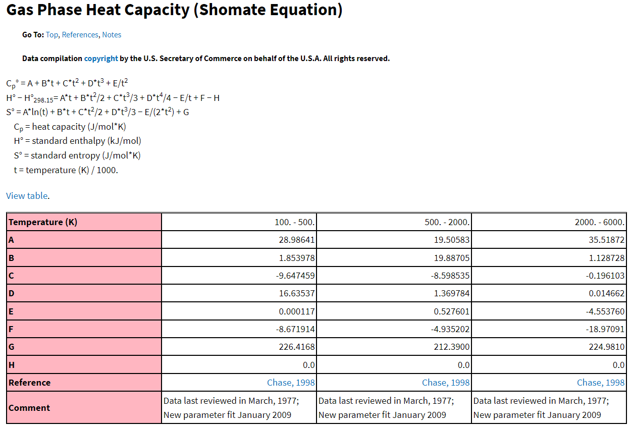
Fig. 6.4 Excerpt from NIST Chemistry WebBook showing fitting parameters to the Shomate Equation for N2 gas. Here, molar specific heat is shown, with the degree symbol indicating that it is molar specific heat at standard conditions of 1 bar and 298.15 K.#
Figure 6.4 shows fitting parameters not only for specific heat, but other thermodynamic properties. Note that although in this figure it is referred to as heat capacity, this is actually molar specific heat, because it is defined per unit mol. Note also the degree symbol, which indicates that this is the molar specific heat capacity at standard conditions, i.e., 1 bar and 298.15 K.
Specific heats are also documented in many other places, for example NIST-JANAF thermochemical tables (https://janaf.nist.gov/). An exerpt is shown below in Figure 6.5, again for N2 gas. Note that these values would be useful if you needed to know the specific heat at a particular temperature, for example if you were assuming it was constant or linear with temperature. Or, from these data you could calculate the Shomate fitting paramaters (or fit your own chosen function), or use to numerically integrate in order to determine changes in enthalpy. Discussion of the other tabulated properties shown here is outside the scope of our discussion for now, but will become relevant later for calculations concerning chemically reacting thermodynamic systems.
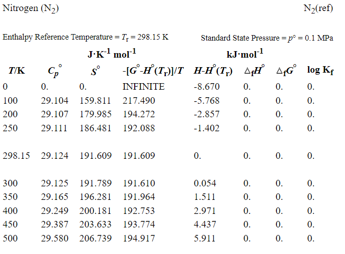
Fig. 6.5 Excerpt from NIST-JANAF Thermochemical Tables showing molar specific heat (and other properties) as a function of temperature. The degree symbol indicates that it is computed at standard conditions of 1 bar and 298.15 K.#
6.5. Relationship between \(c_{\rm p}\) and \(c_{\rm v}\) for Ideal Gases#
At this point, you may have noticed that only specific heats at constant pressure are shown in the NIST databases. There is a straightforward relationship between \(c_{\rm p}\) and \(c_{\rm v}\) that enables computation between one and the other, in the case of ideal gases.
Or in the case of molar specific heats.
This relationship comes from differentiating the equation for enthalpy and subsitutting definitions of \(c_{\rm p}\) and \(c_{\rm v}\), as seen below.
\(h=u+RT\)
\(dh = du+RdT\)
\(c_{\rm p}dT = c_{\rm v}dT+RdT\)
6.6. Using Cantera to Determine \(c_{\rm p}\) and \(c_{\rm v}\) for Ideal Gases#
Of course, since we have learned to use the Cantera package to evaluate thermodynamic properties we can take advantage of its database to evaluate specific heats. When assuming ideal gas behavior, it will be important to calculate specific heats at ambient pressure (e.g. 1 bar) or lower where the calculated values are, for the most part, independent of pressure. This is because the values we have so far learned to extract from Cantera are for real gases, not ideal gases. But, as long as the pressure is sufficiently low there is very little deviation between ideal gas and real gas behavior for most monotonic (e.g. Ar, He) and diatomic gases (e.g., N2, O2).
Now, lets consider how good our assumptions are regarding pressure (or volume) independence of monotonic gases. For this we can call \(c_{\rm p}\) and \(c_{\rm v}\) by following our defined species, in this case nitrogen, with .cp or .cv, such as species1.cp. The units are \(\frac{\rm kg}{\rm J K}\)
import cantera as ct
#State 1
T1,p1,m = 15, 100000, 2 # celsius, Pa, kg
species1 = ct.Nitrogen()# define species1 as nitrogen
species1.TP = 273.15+T1, p1
species1.cp
1040.5742633016914
Now, lets define a list of pressures, from 10 kPa to 100 Mpa and evaluate \(c_{\rm p}\) at each pressure.
import numpy as np
#pressures = 10**np.arange(1,6,1) # alternative approach
pressures = [10**i for i in range(1,6,1)]
cps=[]
for i in pressures:
    species1.TP = 273.15+T1, i
    cps.append(species1.cp)
print(cps)
[1038.784070996967, 1038.7856817302738, 1038.8017891406482, 1038.9628692697945, 1040.574263297144]
As seen, only at the highest pressure of 100 MPa does the specific heat deviate largely from values at lower pressures. And 100 MPa is well above the practical operating pressure for many typical applications. Thus, we can confidently say that for ideal gases specific heats are independent of pressure - and the same conclusion would be drawn if we were to perform calculations as a function of specific volume.
For real gases however, such as water vapor, the pressure (and volume) dependence is greater, as seen below. Although it isn’t until 100 MPa that the deviation becomes very large.
import numpy as np
species1 = ct.Water()
#pressures = 10**np.arange(1,6,1) # alternative approach
pressures = [10**i for i in range(1,6,1)]
cps=[]
for i in pressures:
    species1.TP = 473.15+T1, i
    cps.append(species1.cp)
print(cps)
[1947.2793028311721, 1947.308009567147, 1947.5804720336023, 1950.3244450337818, 1978.3364173330692]
6.7. Determining Changes in Internal Energy or Enthalpy of Ideal Gases using Specific Heats#
As mentioned in Section 6.4 Using Specific Heats with Ideal Gases, there are several aproaches, with varying degrees of accuracy for evaluating internal energy or enthalpy using specific heats. These are
(Least Accurate) Assume specific heat is independent of temperature. In this case \(\Delta u =c_{\rm v} \Delta T\) and \(\Delta h=c_{\rm p} \Delta T\). Typically the specific heat at ambient conditions (e.g. 300 K) is chosen, but if it is known closer to the temperature range of interest then this would result in better accuracy.
(More Accurate) Assume specific heat is linear with temperature and use an average specific heat. In this case \(\Delta u =c_{\rm v,avg} \Delta T\) and \(\Delta h=c_{\rm v,avg} \Delta T\)
(EvenMore Accurate) Determine temperature dependence and integrate analytically using Shomate equation ((8.27)).
The most accurate approach to determining changes in internal energy or enthalpy is to simply use tabulated values or software such as Cantera, which is the equivilent of numerical integration.
We will go through examples of each of these approaches and discuss their accuracy by comparing results to changes in internal energy or enthalpy that are estimated using Cantera. First, let’s take a look at the temperature dependence of \(c_{\rm p}\) of some gases, namely nitrogen, methane and hydrogen. As seen in Figure 6.3, depending on the type of gas, the variability with temperature can change greatly. For example, nitrogen and methane both increase almost linearly with increasing temperature, but \(c_{\rm p}\) of N2 changes only by about 10% while for CH4 it nearly doubles. \(c_{\rm p}\) of H2 is less dependent on temperature, but is a minimum at an intermediate temperature.
Show code cell content
import numpy as np
import cantera as ct
import matplotlib.pyplot as plt
fig=plt.figure()
ax1= fig.add_subplot(1,3,1) # add one subplot
ax2= fig.add_subplot(1,3,2) # add a second subplot
ax3= fig.add_subplot(1,3,3) # add a third subplot
species1 = ct.Nitrogen()# define species1 as nitrogen
species2 = ct.Solution('gri30.yaml')# define species2. Methane does not exist as a class in Cantera so we need to do things a bit differently to define it. See Cantera documentation for more details
species2.X = 'CH4:1' #gri30 is a mixture of gases and here we set the mixture to only be methane
species3 = ct.Hydrogen()# define species3 as Hydrogen
p1 = 100000 #Pa
temperatures = range(300,1000,25) # temperature in degrees C
cps1=[]
cps2=[]
cps3=[]
for i in temperatures:
    species1.TP = i, p1
    cps1.append(species1.cp)
    species2.TP = i, p1
    cps2.append(species2.cp)
    species3.TP = i, p1
    cps3.append(species3.cp)

ax1.plot(temperatures,cps1, label='Nitrogen')
ax2.plot(temperatures,cps2,label='Methane')
ax3.plot(temperatures,cps3, label='Hydrogen')

ax1.set_xlabel('Temperature $(\mathrm{^\circ C})$',  fontsize=12)
ax2.set_xlabel('Temperature $(\mathrm{^\circ C})$',  fontsize=12)
ax3.set_xlabel('Temperature $(\mathrm{^\circ C})$',  fontsize=12)
ax1.set_ylabel('$c_{\mathrm{p}}$ $({\mathrm{kJ kg^{-1}K^{-1}})}$',  fontsize=12)
plt.subplots_adjust(wspace=0.5) # add spacing between subplots
ax1.set_title('Nitrogen')
ax2.set_title('Methane')
ax3.set_title('Hydrogen')
plt.savefig('Figures/cp_temp_depend.png')# used to save the figure if you desire
plt.show()
<>:29: SyntaxWarning: invalid escape sequence '\m'
<>:30: SyntaxWarning: invalid escape sequence '\m'
<>:31: SyntaxWarning: invalid escape sequence '\m'
<>:32: SyntaxWarning: invalid escape sequence '\m'
<>:29: SyntaxWarning: invalid escape sequence '\m'
<>:30: SyntaxWarning: invalid escape sequence '\m'
<>:31: SyntaxWarning: invalid escape sequence '\m'
<>:32: SyntaxWarning: invalid escape sequence '\m'
/tmp/ipykernel_1670/2418094824.py:29: SyntaxWarning: invalid escape sequence '\m'
  ax1.set_xlabel('Temperature $(\mathrm{^\circ C})$',  fontsize=12)
/tmp/ipykernel_1670/2418094824.py:30: SyntaxWarning: invalid escape sequence '\m'
  ax2.set_xlabel('Temperature $(\mathrm{^\circ C})$',  fontsize=12)
/tmp/ipykernel_1670/2418094824.py:31: SyntaxWarning: invalid escape sequence '\m'
  ax3.set_xlabel('Temperature $(\mathrm{^\circ C})$',  fontsize=12)
/tmp/ipykernel_1670/2418094824.py:32: SyntaxWarning: invalid escape sequence '\m'
  ax1.set_ylabel('$c_{\mathrm{p}}$ $({\mathrm{kJ kg^{-1}K^{-1}})}$',  fontsize=12)
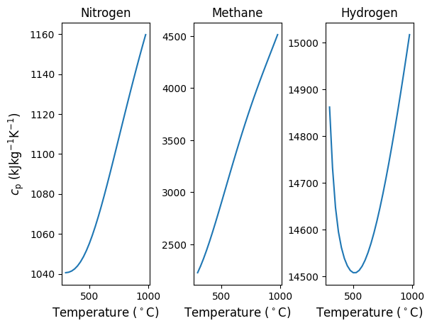
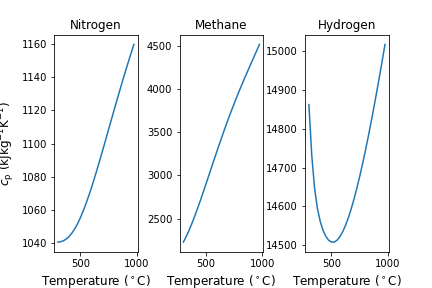
Fig. 6.6 Specific heats of three different gases at ambient pressure, shown as a function of temperature between 300 and 1000 \(^\circ C\). From left to right, Nitrogen, Methane and Hydrogen.#
Thus, from simple visual inspection of Figure 6.6 we can infer that assuming constant \(c_{\rm p}\) will be least accurate for methane, followed by nitrogen and then hydrogen. Further, assuming an average value and a dependence that is linear with temperature will likely be more acceptable for nitrogen and methane compared to hydrogen. Lets compare:
6.7.1. Example - Evaluating Changes in Enthalpy Assuming Constant, Average and Temperature Dependent \(c_{\rm p}\)#
Determine the change in enthalpy of H2 as it is heated from 500 K to 700 K using the three specific heat approaches discussed above. Compare to changes in enthalpy estimated using Cantera.
Solution - First, lets determine the change in enthalpy directly using Cantera. For H2:
import numpy as np
import cantera as ct
T1,T2,P=500,700,100000
species1 = ct.Hydrogen()
species1.TP = T1,P
h1=species1.h
species1.TP = T2,P
h2=species1.h
print("The change in enthalpy is", round((h2-h1)/1000,2), "kJ/kg" )
The change in enthalpy is 2908.91 kJ/kg
Now, using the least accurate, constant specific heat approach. Lets use \(c_{\rm p}\) at ambient conditions, or the default 300 K in Cantera.
import numpy as np
import cantera as ct
T1,T2,P=500,700,100000
species1 = ct.Hydrogen()
cp = species1.cp
print("The specific heat is", round(cp,2), "J/kg/K" )
delta_h=cp*(T2-T1)/1000
print("The change in enthalpy using constant specific heat is", round(delta_h,2), "kJ kg-1" )
The specific heat is 14862.6 J/kg/K
The change in enthalpy using constant specific heat is 2972.52 kJ kg-1
Now, lets calculate the average specific heat and use this to calculate \(\Delta h\).
import numpy as np
import cantera as ct
T1,T2,P=500,700,100000
species1 = ct.Hydrogen()
species1.TP = T1,P
cp1=species1.cp
species1.TP = T2,P
cp2=species1.cp
cp_avg = (cp1+cp2)/2
print("The average specific heat is", round(cp_avg,2), "J/kg/K" )
delta_h=cp_avg*(T2-T1)/1000
print("The change in enthalpy using constant specific heat is", round(delta_h,2), "kJ kg" )
The average specific heat is 14563.59 J/kg/K
The change in enthalpy using constant specific heat is 2912.72 kJ kg
Finally, lets calculate the change in ethalpy through analytical integration of the Shomate equation. We will find the equation from NIST Chemistry Webbook (https://webbook.nist.gov/chemistry/) but can also determine this ourselves, as will be shown in a following, alternative approach after this example. For H2, the Shomate equation is \(c_{\rm p} = A + BT + CT^2 + DT^3 + \frac{E}{T^2}\), with A = 33.066178, B = -11.363417, C = 11.432816, D = -2.772874, and E = -0.158558. To integrate this expression, we can either let Python do this for us using built in functions such as scipy.integrate or it is straightforward to do by hand as well. Both approaches are discussed. First, we will integrate ourselves, as shown below.
\(\Delta h = \int_{1}^{2} c_{\rm p} dT\)
\(\Delta h = \left. AT + \frac{BT^2}{2} + \frac{CT^3}{3} + \frac{DT^4}{4} - \frac{E}{T^{-1}} \right|_{T_1}^{T_2}\)
with the corresponding code
A,B,C,D,E = 33.066178,-11.363417,11.432816,-2.772874,-0.158558
def cp_int(T,A,B,C,D,E): #this is the integrated form of the shomate equation, which we will evaluate at T1 and T2. Units J/mol
    return A*T + B*T**2/2 + C*T**3/3 + D*T**4/4 + E*T**(-1)/(-1)
delta_h=cp_int(700/1000,A,B,C,D,E)-cp_int(500/1000,A,B,C,D,E) # The units are J/mol, as seen from the NIST website. Thus we need to convert to kJ/kg or J/g to compare to our other calculations
M_H2 = 2 # kg/kmol
delta_h=delta_h*1000/M_H2
print("The change in enthalpy using the Shomate Equation is", round(delta_h,2), "kJ/kg" )
The change in enthalpy using the Shomate Equation is 2933.35 kJ/kg
To integrate in Python we can also use the scipy.integrate package and import the quad function, as seen below.
from scipy.integrate import quad
def cp(T,A,B,C,D,E):
    return A + B*T + C*T**2 + D*T**3 + E/(T**2)
delta_h=quad(cp, 500/1000, 700/1000,args=(33.066178,-11.363417,11.432816,-2.772874,-0.158558,)) # Here the args represent our constant. We could have alternatively just let the function cp be dependent on T and inserted these values directly.
delta_h=delta_h[0] # The first output value is the integral and the second is the error. Thus we want only the first value in the output list.
M_H2 = 2 # kg/kmol
delta_h=delta_h*1000/M_H2 # The units were J/mol, as seen from the NIST website. Thus we need to convert to kJ/kg or J/g to compare to our other calculations
print("The change in enthalpy using the Shomate Equation and integrating it with scipy.integrate is", round(delta_h,2), "kJ kg" )
The change in enthalpy using the Shomate Equation and integrating it with scipy.integrate is 2933.35 kJ kg
import numpy as np
import cantera as ct
T1,T2,P=500,700,100000
species1 = ct.Hydrogen()
species1()
  hydrogen:

       temperature   300 K
          pressure   1.0133e+05 Pa
           density   0.081843 kg/m^3
  mean mol. weight   2.0159 kg/kmol
    vapor fraction   1
   phase of matter   supercritical

                          1 kg             1 kmol
                     ---------------   ---------------
          enthalpy             28006             56457  J
   internal energy         -1.21e+06       -2.4393e+06  J
           entropy             64917        1.3087e+05  J/K
    Gibbs function       -1.9447e+07       -3.9204e+07  J
 heat capacity c_p             14863             29962  J/K
 heat capacity c_v             10737             21644  J/K
6.7.2. Example - Evaluating Shomate Equation Knowing Specific Heats as a Function of Temperature#
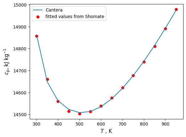
Determine parameters to the Shomate equation for H2 by using the scipy function curve_fit
Solution - First, we need to define our objective function, which is the Shomate Equation.
def shomate(T,A,B,C,D,E):
    return A + B*T + C*T**2 + D*T**3 + E/(T**2)
Then, we need to compile a list of specific heats at different temperatures. For this we will again use Cantera. But these could come from other sources such as NIST-JANAF
import cantera as ct
import numpy as np
species1 = ct.Hydrogen()
temps = np.arange(300,1000,50) #define a temperature list, from 300 K to 100 K every 50 K
cps=[] # create an empy list for cps
for i in temps:
    species1.TP = i,100000 # Everything calculated at 100 kPa
    cps.append(species1.cp)
print(temps)
print (cps)
[300 350 400 450 500 550 600 650 700 750 800 850 900 950]
[14862.565558882909, 14647.86803115975, 14562.046680868487, 14523.003193748402, 14508.210386844778, 14513.200426749348, 14535.061244764198, 14571.105664278139, 14618.976750487958, 14676.655338398828, 14742.430564576087, 14814.860151230303, 14892.730062123708, 14975.01827957901]
Now lets determine the Shomate fitting paramaters by using curve_fit
from scipy.optimize import curve_fit
fit_params=curve_fit(shomate, temps, cps)[0] # The fitted paramaters are the first values from the resulting list, thus we add [0] afterwards
A,B,C,D,E = fit_params
print("Here are the fitted paramaters A,B,C,D and E:", list(fit_params))
Here are the fitted paramaters A,B,C,D and E: [np.float64(12992.693108295514), np.float64(3.233326446376023), np.float64(-0.0027790492760506207), np.float64(1.5308826141905065e-06), np.float64(99342482.54084578)]
fittedcps=[]
for i in temps:
    fittedcps.append(shomate(i,A,B,C,D,E))
print(fittedcps) # These are the fitted specific heats at each temperature in temps
[np.float64(14857.715799511863), np.float64(14660.5194614441), np.float64(14560.242805866303), np.float64(14515.01436967812), np.float64(14503.324269408065), np.float64(14513.465743694434), np.float64(14538.853221799292), np.float64(14575.75575342196), np.float64(14622.119972448712), np.float64(14676.92268601107), np.float64(14739.797256159547), np.float64(14810.80901693958), np.float64(14890.315462351695), np.float64(14978.87651495708)]
import matplotlib.pyplot as plt
plt.plot(temps,cps)
plt.scatter(temps,fittedcps, color='red')
plt.xlabel('$T$ , K',  fontsize=12)
plt.ylabel('$c_\mathrm{p}$, $\mathrm{kJ}$ $\mathrm{kg^{-1}}$',  fontsize=12)
plt.legend(['Cantera','fitted values from Shomate'])
plt.show()
<>:5: SyntaxWarning: invalid escape sequence '\m'
<>:5: SyntaxWarning: invalid escape sequence '\m'
/tmp/ipykernel_1670/1938316306.py:5: SyntaxWarning: invalid escape sequence '\m'
  plt.ylabel('$c_\mathrm{p}$, $\mathrm{kJ}$ $\mathrm{kg^{-1}}$',  fontsize=12)
6.7.3. Exercise 4#
Determine the change in enthalpy of O2 as it is heated from 500 K to 700 K using
property evaluation in Cantera
polynomial expression for specific heat as a function of temperature
average specific heats
constant specific heat at 300 K
A cylinder is fitted with a piston and has an initial volume of 0.1 m3 and contains N2 gas at 150 kPa, 25 °C. The piston is moved, compressing the N2 until the pressure is 1 MPa and T = 150 °C. During compression, heat is transferred from the N2, and the work done on the system is 20 kJ. Determine the amount of heat transfer.
A cylinder is fitted with a piston contains N2 gas at 150 kPa, 25 °C. 300 kJ of heat is transferred to the system at constant pressure. Determine the temperature after heat addition using average specific heats. Note that an iterative solution approach is necessary.
A frictionless piston–cylinder device contains 5 kg of nitrogen at 100 kPa and 250 K. Nitrogen is now compressed slowly according to the relation \(PV\)1.4 = constant until it reaches a final temperature of 450 K. Calculate the work input during this process.
Nitrogen at an initial state of 300 K, 150 kPa, and 0.2 m3 is compressed slowly in an isothermal process to a final pressure of 800 kPa. Determine the work done during this process.
Argon is compressed in a polytropic process with n = 1.2 from 120 kPa and 30°C to 1200 kPa in a piston–cylinder device. Determine the final temperature of the argon.
Determine the change in specific internal energy of hydrogen as it is heated from 200 to 800 K using a) the Shomate specific heat equation as a function of temperature, b) using an average cv value, c) using a room temperature cv value, and d) using Cantera.
1 kg of oxygen is heated from 20 to 120°C. Determine the amount of heat transfer required when this is done during both a constant-volume process and an isobaric process. For each use
specific heat equation as a function of temperature
using an average cv value
using a room temperature cv value
using Cantera.
Argon (cv = 0.3122 kJ/kg/K) is compressed in a polytropic process with n = 1.2 from 120 kPa and 10°C to 800 kPa in a piston–cylinder device. Determine the work produced and heat transferred during this compression process, in kJ/kg.
A piston–cylinder device contains 2.2 kg of nitrogen initially at 100 kPa and 25°C. The nitrogen is now compressed slowly in a polytropic process during which \(PV\)1.3 = constant until the volume is reduced by one-half. Determine the work done and the heat transfer for this process.
1kg of nitrogen undergoes a polytropic process with n = 2. The nitrogen compresses to one third of its original volume and ends at T = 750 K. What is the inital temperature (T) and work (W) done in this process?
Carbon Dioxide is heated from T = 350 K to T = 500 K. 115 kJ of heat is added to the gas during this process. What is the molar average specific heat (Cv) during this heating?
Nitrogen is heated from T = 400 K to T = 750 K in a rigid container. Assume nitrogen is an ideal gas.
What is the change in specific internal energy (u) using average specific heat?
What is the change in specific internal energy (u) using cantera values?
Carbon dioxide undergoes a polytropic process from T2/T1 = 3 and V1/V2 = 2. What is the work (W) done per kg during this process if the intial temperature is T = 300 K?
Determine the change in specific internal energy (u) of hydrogen when it is heated from T = 400 K to T = 500 K.
Using an average cv value.
Using a room temperature cv value.
Using cantera.