8. Second Law of Thermodynamics - Directionality of Processes, Entropy, Heat Engines and Refrigerators

So far, we have focused our attention on evaluating properties of substancies (e.g., enthalpy, volume) using various techniques and evaluating processes by applying the First Law of Thermodynamics, or conservation of energy. And we know that if the First Law of Thermodynamics is not satisfied then a process or cycle is not possible. Yet, there are numerous situations where the First Law of Thermodynamics is satisfied but the process is still not possible. For example, consider a closed system with a paddle wheel contained within it. We know from experience that if we do work to the system by rotating the paddle wheel, that the system will heat up, its internal energy will increase, etc. Yet, the reverse will not happen - i.e., we cannot heat up the system and spontanesouly expect the paddle wheel to rotate, resulting in work done by the system. Yet this in no way would violate the first law of thermodynamics. This implies that there is a directionality associated with processes that is important, and it is the directionality of a process that is the realm of the Second Law of Thermodynamics. Thus, the Second Law of Thermodynamics adds further constraints to processes on top of the First Law. In fact, we will learn that no real process will happen spontaneously without an increase in a thermodynamic property which we will learn about called entropy (\(S\)). Simply put, entropy must always be increased for a process to occur (or for a reversible process, which is not possible in reality, entropy remains unchanged). Entropy can be thought of as a driving force for energy exchange - i.e, if it can be increased then energy transfer will occur. It is because of the Second Law that heat always flows from hot reservoirs to cold reservoirs, that pressures tend to equalize and that gases mix. In all of these cases we can show that entropy increases as a result. This is not to say that entropy cannot be decreased locally, but only that the total entropy of the control volume (i.e., the system) and the surroundings must be increased for a process to occur. As a result, the second law of thermodynamics is sometimes referred to as the increase in entropy principle.

In the remainder of this chapter will will motivate the idea of process directionality from a qualitative perspective and build on the concept of entropy and increasing entropy (or entropy generation) as a necessary condition for a process to occur. In later chapters we will build a mathematical framework for the description of entropy.

8.1. Directionality - Qualitative Motivation through Heat Engine Thermodynamic Cycles

As mentioned prior, we are already innately aware that there is a directionality to processes. Energy always flows from hot to cold, which really means from low entropy to high entropy - if the reverse were true then your cup of hot coffee would continue to increase in temperature and the surroundings would cool. Gases that are well mixed such as nitrogen and oxygen do not spontaneously separate, and so on. This directionality has profound influences on thermodynamic processes and cycles and can be exemplified through the introduction of a heat engine. A heat engine operates on a thermodynamic cycle and is a device that takes advantage of the flow of heat to produce work. Now, when we mention the production of work within the context of a thermodynamic cycle, which we have learned prior means that we start and end at the same thermodynamic state, what we really mean is the net production of work resulting from the thermodynamic cycle. The entire framework for the Second Law of Thermodynamics was originally conceived by Sadi Carnot, who developed the concept of a heat engine and who at the time had no concept of entropy as a thermodynamic property. Yet, he recognized that it is impossible for any heat engine that operates on a cycle to produce a net amount of work without absorbing heat from the surroundings at a high temperature and rejecting a portion of it back to the surroundings at some lower temperature. That is, it is impossible to convert 100% of heat into work if operating on a cycle, and the direction of heat flow is from hot to cold. A schematic of an impossible process can be seen on the left side of Figure 8.1, where there is no heat rejection and thus no net work can be produced. Rather, some portion of the heat must be rejected at a lower temperature, as seen on the right side of Figure 8.1. And Carnot further observed that heat has an innate quality tied to it that is related to the heat engine efficiency, that is, the higher the temperature heat source the more efficient the heat engine can operate - we will learn later that this quality is closely tied to entropy. Carnot’s insights eventually formed the framework for one variation of the Second Law which is called the Kelvin-Plank statement. The Kelvin-Plank statement states that “It is impossible to construct a device that will operate in a cycle and produce no effect other than the raising of a weight and the exchange of heat with a single reservoir”.

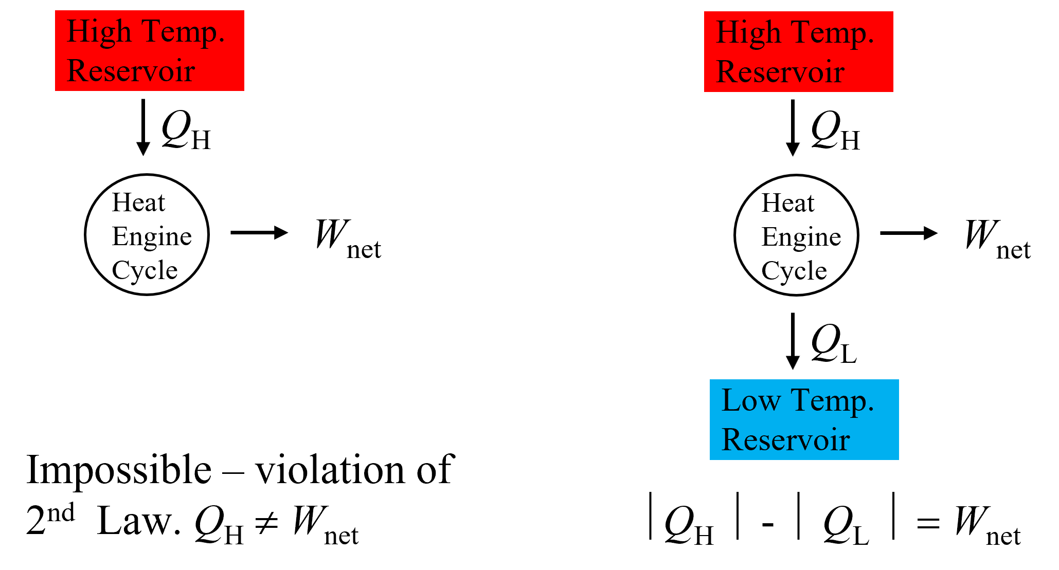
Fig. 8.1 An example of an impossible process (left) which violates the second law of thermodynamcs because 100% of thermal energy cannot be converted to work. Rather, some smaller portion of the incident energy must be rejected at a lower temperature, as seen on the right side.

The process of converting heat into work via a heat engine and two thermal reservoirs can be imagined similarly to a turbine producing work from the flow of liquid (e.g. a waterfall). If we wish to extract work from the potential energy of water at a high elevation, we can use a turbine, but we still must release the water at some lower elevation (and lower potential energy). Otherwise, the exiting fluid would quickly rise in elevation, and an equilibrium would be established such that the exit and inlet heights are the same and the turbine ceases to rotate. Thus, just as fluid flow will always spontaneously occur from high elevation to low elevation, but never the reverse, heat flow will always spontaneously travel from high temperature to low temperature. And if we wish to extract work we must still reject some portion of the energy flow at a lower quality than the inlet.

Let’s conceptualize why this must be true. Imagine a cycle that starts in one state, for example at given temperature, and we aim to extract energy in the form of work by adding heat to the system. For example, we could heat a piston filled with a gas and it will expand, producing work. An example is shown below in Figure 8.2 where in the first 4 iterations we raise a mass (shown in green) to a higher elevation. Yet, to complete the cycle, we will have to get back to our original state. One way to do this would be to follow the same path that we took to extract the work, by replacing the mass and then rejecting heat at the same high temperature (shown in the remaining iterations in Figure 8.2) but then this would mean that the same amount of energy we got out in the form of work would have to be put back into the process (assuming both were reversible). Thus there would be no net production of work and our heat engine will not operate.

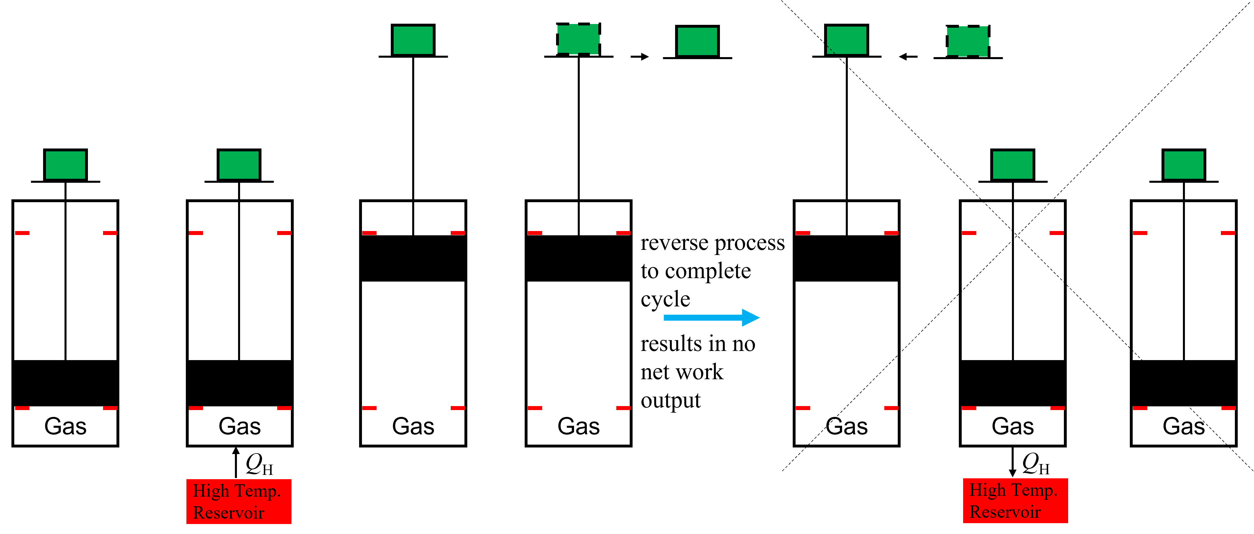
Fig. 8.2 An example of an impossible process heat engine.

This means that we must take a different path back to return to our original state if we want the chance of producing a net amout of work. What the system would have to do, it turns out, is to reject heat, and then compress the piston along a different path to get back to our original state. This is shown in Figure 8.3, where he piston is lowered first by rejecting heat to a low temperature reservoir. Then, to return to our initial state we can further compress the system by adding the mass back to the top of the piston, but from a lower elevation that before, thus requiring less work. In this way, we can decrease the work requirements to return to our original state, resulting in some net production of work. There are only two ways to impact the state of the system (and internal energy, volume, entropy etc) - through work or heat exchange - and by rejecting heat at a lower temperature instead of doing work following expansion, we can also locally decrease the energy and entropy of the system to help approach its initial value. The inevitable result is that if we return to our original state that the entropy (and energy, volume, etc) remain unchanged within the control volume, and thus the entropy will have to increase in the surroundings (unless we had a completely reversible heat engine). More on this later.

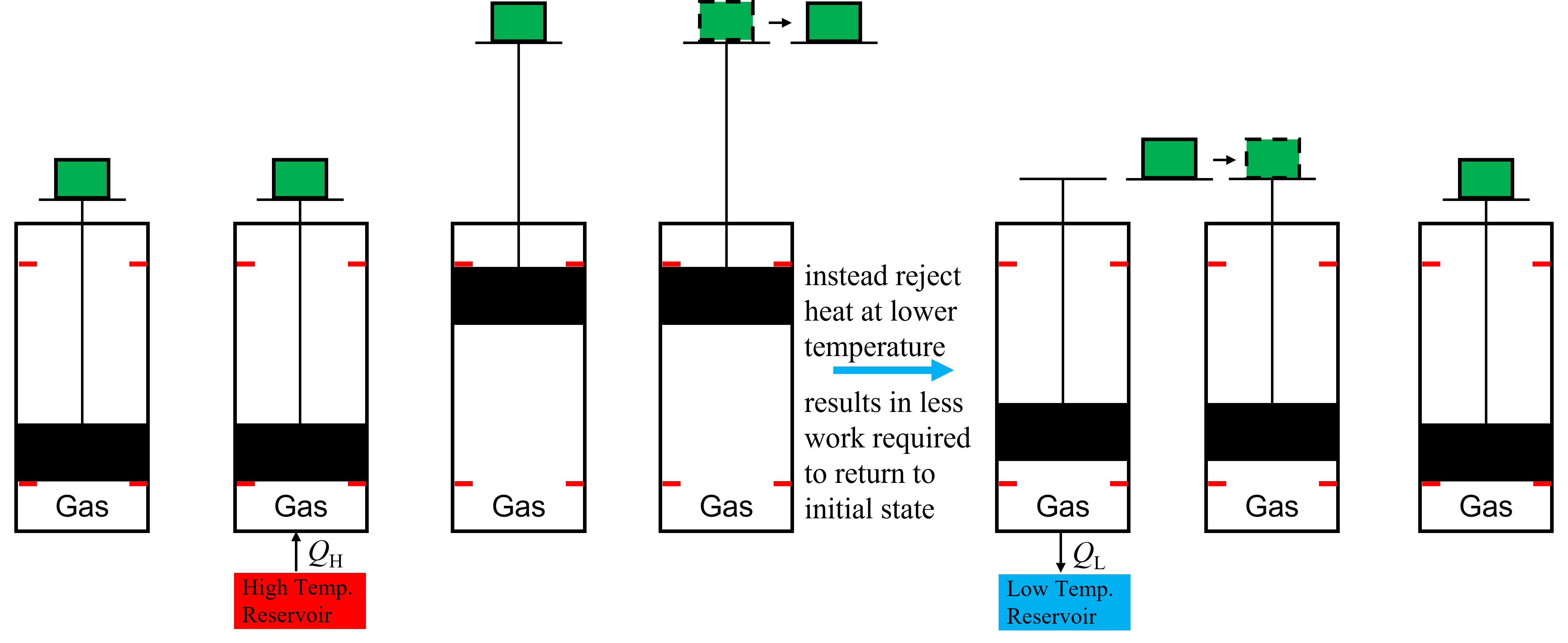
Fig. 8.3 An example of a simple heat engine that works by rejecting heat at a lower temperature than it is absorbed.

8.2. Directionality - Entropy is Multiplicity Maximization

And now the logical questions is, why must heat always flow from hot to cold in a spontaneous process, and not vice versa? Why should gases spontaneously mix and not separate, why do gases expand in closed systems, and why do chemical reactions spontaneously occur in one direction but not the reverse, for example the combustion of hydrocarbons even if energy is conserved in an adiabatic chamber. The reason for this, in all of the above cases and more, is that the entropy is maximized. And whenever there is the potential to increase entropy, a process will spontaneously occur (given sufficient time). Then the next logical question is, what is entropy? Although you may have learned prior it is a measure of disorder of the system (and this analogy can be useful), a better explanation, I think, is that entropy is simply related to the number of possible ways a system can be arranged or configured from a microscopic perspective, referred to as the multiplicity (\(W\)) of the system. It is purely a statistical phenomenon - the system will always tend towards the state in which it can be arranged the greatest number of ways. For example, lets consider why gases tend to want to disperse. If we have a system of two particles (e.g., gas molecules) which can be distributed in any of 4 different boxes like shown below in Figure 8.4 (imagine the number of boxes is related to the volume of the system), it is statistically more probable to find them in separate boxes rather than in the same. There are 4 configurations we can envision in which they are the same box (left side) and 6 in which they are separated (right side). And as the number of boxes increases, the chances that they are found in the same box become less probable. For example, if the number of boxes increased to 8, then there are only 8 configurations where they can be in the same box but 28 where they are different. When considered on the scale of real systems, with orders of magnitude more molecules, the probability of finding the molecules in a configuration not well dispursed becomes vanishingly small as the multiplicity increases. And thus from a statistical perspective, there are many more configurations available in which the molecules are well dispersed rather than confined near each other. Interestingly, this approach does not assume that it is impossible that the molecules remain in a clumped together configuration - is only statistically improbable. That is, the most statistically probable configuration is the one which is most likely to occur, and the most statistically probable outcome is the one with the largest number of possible configurations. Entropy is simply a measure of the number of ways we can arrange a system and thus this tends to want to be maximized because it is statistically more probable. Another way to think about multiplicity is that as it increases, our our uncertainty about the location of the molecules decreases. We can decscribe the multiplicity of a system (\(W\)) mathematically as

(8.1)\[W = \frac {N!}{n_{\rm {1}}!n_{\rm {2}}!...n_{\rm {i}}!}\]

where \(N\) is the number of objects (in this case boxes) with i categories (in this case a box is either empty or not, so two categories). For example, in the case of both particles contained in the same box only 1 is not emtpy, thus, \(N\) = 4, \(n_\rm {1}\) = 1 and \(n_\rm {1} = 3\). For the case of finding both particles in separate boxes, only 2 are empty, and thus, \(N\) = 4, \(n_\rm {1}\) = 2 and \(n_\rm {1} = 2\).

Fig. 8.4 Why do gases tend to disperse rather than clump together? There are more ways to arrange the system in the latter case, thus the multiplicity, and entropy are greater. As seen on the left, there are 4 ways to arrange 2 gas molecules both in the same cube, with the remaining 3 empty. But if two are filled and two empty (more dispersed), when we can arrange the system 6 ways. Thus, the multiplicity of the latter is greater, thus also the probability that this outcome will occur. Entropy is simply a measure of the multiplicity - the system will more likely be in the configuration that maximizes multiplicity (because it is statistically more probable). So to will the entropy always be maximized.

A slighty more complex example can be used to show why heat flows from hot to cold - as you may have guessed it is because entropy is maximized. For this example, lets consider two separate and isolated systems, A and B, that are brought into thermal contact and allowed to exchange heat, as illustrated below in Figure 8.5. The internal energy of these systems are dictated by 1) the number of particles (e.g., gas molecules) in the system and 2) whether or not those particles are energized (\(\epsilon\)). For this example we are considering only very simplified systems with only a limited number of particles and limited energy states equal to only 0 or 1. System A is initially composed of 5 particles (\(N_\rm {A} = 5\)) with internal energy (\(U_\rm {A} = 2\)) and System B is initially composed of 5 particles (\(N_\rm {A} = 5\)) with internal energy (\(U_\rm {A} = 4\)), shown schematically on the top of Figure 8.5. Note that because the particles can only have energies of 0 or 1, system A must have two energized particles and system B must have 4. We can calculate the multiplicity to see the number of ways in which we can arrange each of these systems, according to (8.1), and we see that for System A, \(W\)_A = 10 and for System B, \(W\)_B = 5. Now, initially Systems A and B cannot exchange heat but we can consider the total multiplicity of the combined systems by drawing a control volume around both systems, shown in the green dash-dotted line. For the combined number of configurations it is simply the product of each (e.g., 10 configurations of A with the 1st of B, 10 configurations with the 2nd, and so on). So, the total multiplicity for systems A and B is 50.

Now, if the adiabatic barrier between A and B is removed and energy can be exchanged, then the internal energy of each system can change but the total internal energy of the combined systems must remain constant (\(U_\rm A\) + \(U_\rm B\) = 6). We could imagine a scenario where the internal energy of A decreases to 1 and B increases to 5, in which case \(W\)_A = 5 and \(W\)_B = 1 and thus \(W\)_total = 5 which is lower than the initial value. Thus, this is not statistically probable and therefore the energy flow will likely not be from cold to hot. However, consider the reverse case of heat transfer from hot to cold, in which case the internal energy of A could increase to 3 and of B could decrease to 3. This scenario is shown on the bottom of Figure 8.5. In this scenario, \(W\)_A = 10 and \(W\)_B = 10 and thus \(W\)_total = 100 which is greater than the initial value of 50. Thus it is statistically more probable that energy will flow from the hotter system B to the lower temperature system A. Although we have only shown a few scenarios, ultimately the energies of each system will be determined by maximizing the multiplicity by considering all possible scenarios - however it turns out that the final condition considered here is where multiplicity is maximized. Thus, we can see that energy tends to want to flow from hot to cold (i.e., in this case higher specific internal energy to lower) and it does so because there are more ways to configure the system. Thus, it is statistically more probable that this occurs. And as mentioned, entropy is a measure of the multiplicity of the system and since this tends to want to increase, the entropy as well can be considered to want to increase.

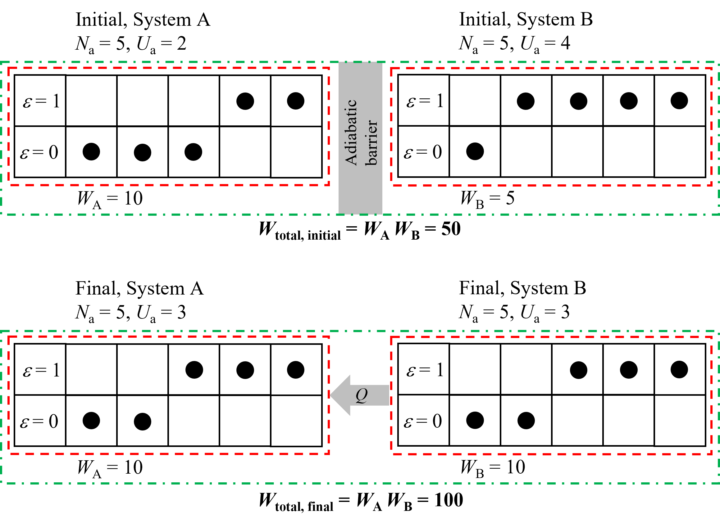
Fig. 8.5 An example showing why energy tends to want to flow from higher temperature to lower. On the top two systems are isolated with different internal energies (i.e., different temperatures) and the total multiplicity of the combined systems is 50. When we allow energy to transfer by removing the adiabatic barrier, as shown on the bottom, the multiplicity is increased when the internal energy of B decreases and A increases. Thus, there are more ways to arrange this system and therefore it is more statistically probably. Thus, we can see the multiplicity and thus entrpoy increase if energy flows from hot to cold. In the reverse case the multiplicity and entropy would decrease below the initial value, which is statistically improbable.

This insight leads to a different variation of the second law of thermodynamics - i.e., there is no process which results only in the transfer of heat from a cold reservoir to a hot reservoir. For this to be possible, work from an external source would have to be done to the system. This is commonly referred to as a heat pump, or refrigeration cycle. This was first formulated as the Clausius Statement. It states that “It is impossible to construct a device that operates in a cycle and produces no effect other than the transfer of heat from a cooler body to a warmer body.” And from our statistical example above, we know that the reason for this has to do with multiplicity, or entropy, and its tendancy to be maximized.

8.3. Thermodynamic Driving Forces

Now, at this point we have shown that multiplicity tends to increase for spontaneous processes - i.e. as processes go towards equilibrium their multiplicity increases. Further, we have said that multiplicity is a measure of entropy - but this has not been proven. Specifically, for now let’s postulate the following since as of yet entropy has not been definied explicitly.

(8.2)\[S \propto W\]

We have shown that \(W\) depends on volume (\(V\)) and internal energy (\(U\)). For example, W increases as N (e.g., the number of boxes in Figure 8.4, or volume) increases, keeping the number of particles constant. Further, W decreases as the internal energy decreases, also keeping the number of particles constant, as was shown in Figure 8.5. We can also shown that \(W\) is a function of the number of particles in the system. For example, imagine in Figure 8.5 that System A was initially composed of 6 particles instead of 5, with the same total internal energy. With 6 particles the multiplicity is 120 versus only 10 in the case of 5 particles. Thus, we can say the the multiplicty is a function of \(U\), \(V\) and the number of particles \(N\)_a, or

(8.3)\[W = f(U,V,N_{\rm a})\]

and because \(S \propto W\)

(8.4)\[S = f(U,V,N_{\rm a})\]

For the time being we will consider only systems where the number of particles remains constant to simplify analysis. Further, all of our prior examples of thermodynamic systems were such that \(N\)_a = constant. I.e., they were constant mass and there were no chemical reactions considered that could change the number of moles. Thus we can say the following for \(N\)_a = constant.

(8.5)\[S = f(U,V)\]

Taking the derivitive we can see how this depends on variations of the independent properties \(U\) and \(V\).

(8.6)\[dS = \left( \frac{\partial S}{\partial U} \right)_{\rm V} dU + \left( \frac{\partial S}{\partial V} \right)_{\rm U} dV\]

With this as a starting framework, lets evaluate two different processes as they approach equilibrium. For this we will make one important assumption, of which we can later test the validity. This assumption is that the entropy is an extensive thermodynamic property of the system, and therefore dependent on the system size, just like internal energy and volume. We know that extensive thermodynamic properties are additive.

8.3.1. Process 1 - Constant Volume Equilibration

Consider two separate systems, A and B, as shown in Figure 8.6 initially at different temperatures and internal energies, both with fixed volumes, separated by an adiabatic barrier. Then, the barrier is now diathermal and allowed to transfer heat until the total combined system (A + B) is equilibrated. We know from our prior example that at equilibrium, entropy is maximized and thus we can say that at the final state \(dS = 0\). Further, because each of the subsystem volumes are constant, then the total system volume must also be constant, or \(dV = 0\).

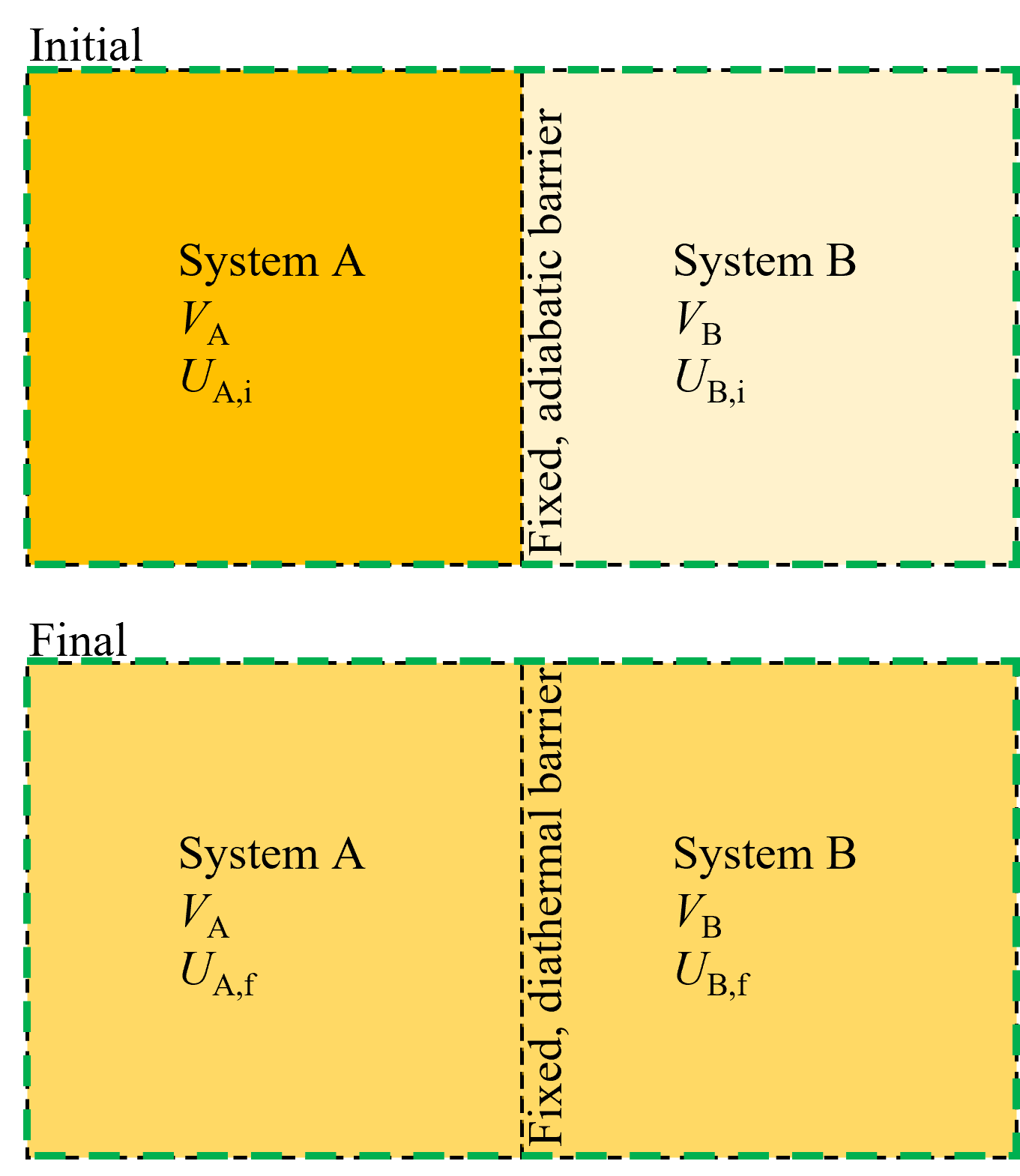
Fig. 8.6 For two fixed volume systems that are initially isolated and then allowed to exchange heat, it is equilibration of temperatures that dictates equilibrium.

Conservation of energy states that the total internal energy of A and B must remain constant, and that the energy gained in one is lost in the other, i.e.

(8.7)\[(U_{\rm A,i} + U_{\rm B,i} = U_{\rm A,f} + U_{\rm B,f} = const.)\]

(8.8)\[U_{\rm A,i} - U_{\rm A,f} = U_{\rm B,f} - U_{\rm B,i}\]

(8.9)\[\Delta U_{\rm A} = -\Delta U_{\rm B}\]

and

(8.10)\[d U_{\rm A} = -d U_{\rm B}\]

Starting from (8.6), recognizing \(dV = 0\) for each sub-system, as we approach equilibrium we can say for each of our two systems that

(8.11)\[dS_{\rm A} = \left( \frac{\partial S_{\rm A}}{\partial U_{\rm A}} \right)_{\rm V} dU_{\rm A}\]

(8.12)\[dS_{\rm B} = \left( \frac{\partial S_{\rm B}}{\partial U_{\rm B}} \right)_{\rm V} dU_{\rm B}\]

And because of our assumption that entropy is an extensive thermodynamic property, the total system entropy at equilibrium is

(8.13)\[dS = dS_{\rm A} + dS_{\rm B} = 0\]

Substituting from above

(8.14)\[\left( \frac{\partial S_{\rm A}}{\partial U_{\rm A}} \right)_{\rm V} dU_{\rm A} + \left( \frac{\partial S_{\rm B}}{\partial U_{\rm B}} \right)_{\rm V} dU_{\rm B} = 0\]

and substituting (8.10)

(8.15)\[\left( \frac{\partial S_{\rm A}}{\partial U_{\rm A}} \right)_{\rm V} dU_{\rm A} - \left( \frac{\partial S_{\rm B}}{\partial U_{\rm B}} \right)_{\rm V} dU_{\rm A} = 0\]

This can be rearranged to show

(8.16)\[dU_{\rm A} \left [ \left( \frac{\partial S_{\rm A}}{\partial U_{\rm A}} \right)_{\rm V} - \left( \frac{\partial S_{\rm B}}{\partial U_{\rm B}} \right)_{\rm V} \right] = 0\]

In other words, at equilibrium

(8.17)\[\left( \frac{\partial S_{\rm A}}{\partial U_{\rm A}} \right)_{\rm V} = \left( \frac{\partial S_{\rm B}}{\partial U_{\rm B}} \right)_{\rm V}\]

Now, this begs the question - what thermodynamic property of system A and system B are equal to each other at equilibrium that could represent the partial differentials that must be equal? The answer is intuitive - temperature! The thermodynamic property that is a driving force for energy exchange is temperature, not internal energy, volume, etc. Therefore, we can say that

(8.18)\[\frac{1}{T}=\left( \frac{\partial S}{\partial U} \right)_{\rm V}\]

or more generally

(8.19)\[\frac{1}{T}=\left( \frac{\partial S}{\partial U} \right)_{\rm V, N_a}\]

The reason that temperature is inverted has to do with the fact that we know enrgy flow must be from hot to cold and the entropy maximized. If instead we said \(T=\left( \frac{\partial S}{\partial U} \right)_{\rm V, N_a}\), the entropy change towards equilirium dS would be negative unless the energy flow were from cold to hot. You can convince yourselve with a quick calculation. Thus, we can say for fixed volume systems, temperature is the driving force for heat exchange and that it is equalized when the system reaches equilibrium.

8.3.2. Process 2 - Variable Volume Equilibration

Consider two separate systems, A and B, as shown in Figure 8.7 initially at different temperatures and internal energies, separated by an adiabatic fixed barrier. Then, the barrier is allowed to conduct heat and move, enabling system A and B to exchange heat and work (but not with the surroundings) until the total combined system (A + B) is equilibrated. Again, we know from our prior example that at equilibrium entropy is maximized and thus we can say that at the final state \(dS = 0\).

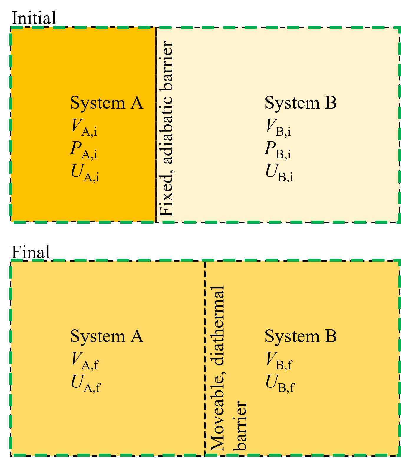
Fig. 8.7 For two systems that are initially isolated and then allowed to exchange heat and work via a diathermal and movable membrane, equilibrium occures when the temperature and pressure of each side are equaized.

Conservation of energy states that the total internal energy of A and B must remain constant, and that the energy gained in one is lost in the other, i.e.

(8.20)\[(U_{\rm A,i} + U_{\rm B,i} = U_{\rm A,f} + U_{\rm B,f} = const.)\]

(8.21)\[U_{\rm A,i} - U_{\rm A,f} = U_{\rm B,f} - U_{\rm B,i}\]

(8.22)\[\Delta U_{\rm A} = -\Delta U_{\rm B}\]

, and

(8.23)\[d U_{\rm A} = -d U_{\rm B}\]

Because the total volume of the combined systems is constant we can also say that

(8.24)\[d V_{\rm A} = -d V_{\rm B}\]

Thus, starting from (8.6), as we approach equilibrium we can say for each of our two systems that

(8.25)\[dS_{\rm A} = \left( \frac{\partial S_{\rm A}}{\partial U_{\rm A}} \right)_{\rm V_A} dU_{\rm A} + \left( \frac{\partial S_{\rm A}}{\partial V_{\rm A}} \right)_{\rm U_A} dV_{\rm A}\]

(8.26)\[dS_{\rm B} = \left( \frac{\partial S_{\rm B}}{\partial U_{\rm B}} \right)_{\rm V_A} dU_{\rm B} + \left( \frac{\partial S_{\rm B}}{\partial V_{\rm B}} \right)_{\rm U_B} dV_{\rm B}\]

And because of our assumption that entropy is an extensive thermodynamic property, the total system entropy at equilibrium is

(8.27)\[dS = dS_{\rm A} + dS_{\rm B} = 0\]

Substituting (8.25) and (8.26) into (8.27), then substituting (8.23) and (8.24) and rearranging we can see that

(8.28)\[\left[ \left( \frac{\partial S_{\rm A}}{\partial U_{\rm A}} \right)_{\rm V_A} - \left( \frac{\partial S_{\rm B}}{\partial U_{\rm B}} \right)_{\rm V_A} \right]dU_{\rm A} + \left[\left( \frac{\partial S_{\rm A}}{\partial V_{\rm A}} \right)_{\rm U_A} -\left( \frac{\partial S_{\rm B}}{\partial V_{\rm B}} \right)_{\rm U_B} \right]dV_{\rm A} =0 \]

We know that at equilibrium the left hand terms equal zero because \(T_{\rm a}\) = \(T_{\rm b}\) and \(\frac{1}{T}=\left( \frac{\partial S}{\partial U} \right)_{\rm V}\). Therefore the terms \(\left( \frac{\partial S}{\partial V} \right)_{\rm U}\) for systems A and B must also be equal. Does this partial differential also equal some measurable property like in the prior example where \(\frac{1}{T}=\left( \frac{\partial S}{\partial U} \right)_{\rm V}\)? To see, let’s first consider the units of entropy. We know that \(\frac{1}{T}=\left( \frac{\partial S}{\partial U} \right)_{\rm V}\), and thus S has units kJ/K. Thus entropy per unit volume should have units kJ/K/m³. This can be rearranged as kN/m²/K which is the same units as we would expect for the ratio of properties, \(p/T\). And therefore, not surprisingly it turns out that \(\left( \frac{\partial S}{\partial V} \right)_{\rm U} = \frac{p}{T}\). That is, equilibration between systems with a diathermal and movable barrier results in the equality of the ratio of temperature to pressure. Physically, this make sense, as we intuitively know that the system at equilibrium should have equal temperatures and pressures.

8.4. Thermodynamic Definition of Entropy

Recall that we started with the discussion above with the assumption that entropy is proportional to multiplicity, and thus a function of energy and volume, or

(8.29)\[S = f(U,V)\]

We then took the derivitive of this function and saw that

(8.30)\[dS = \left( \frac{\partial S}{\partial U} \right)_{\rm V} dU + \left( \frac{\partial S}{\partial V} \right)_{\rm U} dV\]

Which reduces to the following because \(\left( \frac{\partial S}{\partial U} \right)_{\rm V} = \frac{1}{T}\) and \(\left( \frac{\partial S}{\partial V} \right)_{\rm U} = \frac{p}{T}\).

(8.31)\[dS = \frac{1}{T} dU + \frac{p}{T} dV\]

Now, consider a reversible expansion or compression process of an ideal gas. Recall from Section 6.1 More on Boundary Work - Reversible Processes that a reversible process is one in which occurs very slowly and is not possible in reality - but it represents an ideal process. We can relate the reversible boundary work (\(\delta W_{\rm rev}\)) to \(pdV\), or

(8.32)\[\delta W_{\rm rev} = pdV\]

We also know from the First Law of Thermodynamics that

(8.33)\[dU = \delta Q_{\rm rev} - \delta W_{\rm rev}\]

Thus, we we can substitute (8.32) and (8.33) into (8.31) to show that

(8.34)\[dS = \frac{1}{T} (\delta Q_{\rm rev} - \delta W_{\rm rev}) + \frac{\delta W_{\rm rev}}{T}\]

or

(8.35)\[dS = \frac{1}{T} \delta Q_{\rm rev}\]

and also

(8.37)\[\delta Q_{\rm rev} = TdS \]

Now, although there are infinite number of pressure volume temperature paths that we could take to go from State 1 to State 2 (and thus varying degrees of reversible work), the change in entropy is only dependent on the heat transfer to or from the system. This is significant because it ties the entropy change of the system to a measureable quantity, namely the heat transfer, rather than relating it to probabiities or multiplicity which is not readily measurable. Also, significantly, it shows that the entropy of the system can be increased or decreased, depending on the direction of heat transfer, lending credence to the idea that entropy can be decreased locally at a system level, which partly explains how order can rise from apparant disorder.

8.4.1. Example - Evaluating Reversible Heat Transfer Using Entropy

A piston cylinder maintaining constant pressure contains 0.1 kg saturated liquid water at 100°C. It is now boiled to become saturated vapor in a reversible process. Find the work term and then the heat transfer from the energy equation. Find the heat transfer from the entropy equation, is it the same?

Solution - If using the energy equation, for a closed system like this, \(\Delta U = Q_{\rm net}- W_{\rm net}\), and because this is a constant pressure process \(W_{\rm net}=P \Delta V\). Thus, the heat transfer can be solved knowing internal energy and volume at the initial and final states. Or, more simply we can also say \(Q_{\rm net}=\Delta H\) because the process is constant pressure. We can use Cantera to solve.

If using the entropy equation from above (8.37), \(\delta Q_{\rm rev} = TdS\), this can be readily integrated because the process occurs at constant temperature. Thus \(Q_{\rm rev} = T \Delta S\). Thus, we need only the entropy at the initial and final states. We can use Cantera to solve.

import cantera as ct
#State 1
m= 0.01 #kg
T1 = 100 + 273.15 #K
x1 = 0 # Sat. Liquid

species1 = ct.Water()# define state 1
species1.TQ = T1, x1

#State 2
T2=T1 #K
x2 = 1 # Sat. Liquid

species2 = ct.Water()# define state 2
species2.TQ = T2, x2

dh=species2.HP[0]-species1.HP[0]
ds=species2.SP[0]-species1.SP[0]

print(round(dh*m,2), "J, is Q using the Energy Equation")
print(round(ds*m*T1,2), "J, is Q using the Entropy Equation")

22570.44 J, is Q using the Energy Equation
22570.44 J, is Q using the Entropy Equation

8.5. Entropy Generation

We have just stated that entropy can decrease locally, but this is seemingly at odds with the fact that the second law of thermodynamics earlier in this chapter was motivated by saying that any spontaneous process that tends toward equilibrium must result in an increase in entropy. At this point, it is important to consider the distinction between the system and surroundings, and that when we say entropy must always increase, this refers to the total, or combined, entropy of the system and surroundings. Thus, if the entropy of a system decreases (for example by rejecting heat), then the entropy of the surroundings must increase by at least as much, and even more unless the process were reversible. We can see why entropy must always be increased (or generated) in a real process by comparing it to a reversible one. Lets first consider the reversible and adiabatic expansion process between states 1 and 2, as shown on the left of Figure 8.8. Because it is adiabatic there is no heat transfer and so the change in entropy according to (8.35) is zero. If the expansion process is real (i.e., irreversible) and to the same pressure, then the path taken is different and the work is less. According to the conservation of energy equation, if the work is less, the change in internal energy is less and thus, the temperature change should also be less compared to the reversible process. Thus, \(T\)₃ > \(T\)₂. Now, the only way to get to State 3 from State 2 is to reject heat from the system. Considering entropy is a state property and doesn’t depend on the path, then \(S\)₂-\(S\)₁ = \(S\)₂-\(S\)₃ + \(S\)₃-\(S\)₁. Since \(S\)₂-\(S\)₁ = 0 (reversible and adiabatic) and \(S\)₂-\(S\)₃ < 0 because of (8.35) and the heat transfer is negative (i.e. heat rejection), then \(S\)₃-\(S\)₁ must be positive and thus \(S\)₃ > \(S\)₁. Entropy was generated during the irreversible and adiabatic expansion process!

Fig. 8.8 Entropy is generated for both expansion and compression processes that are irreversible. All irreversible processes result in entropy generation.

Now, lets consider the reverse case. I.e., reversible and adiabatic compression versus irreversible and adiabatic compression, as shown on the right of Figure 8.8. In this case the temperature following irreversible compression will be greater than the reversible case because the work requirement will be greater and according to the first law the internal energy change must be greater. This compression process is shown going from State 2 to State 3a. Then, the only way to return back to State 1 is to again reject heat from the system. Again considering entropy is a state property and doesn’t depend on the path, then \(S\)₁-\(S\)₂ = \(S\)_3a-\(S\)₂ + \(S\)₁-\(S\)_3a. Since \(S\)₁-\(S\)₂ = 0 (reversible and adiabatic) and \(S\)₁-\(S\)_3a < 0 because of (8.35) and the heat transfer is negative (i.e. heat rejection), then \(S\)_3a-\(S\)₂ must be positive and thus \(S\)_3a > \(S\)₂. Entropy was also generated during the irreversible and adiabatic compression process! And in fact, the entropy change must always increase for an irreversible process.

Mathematically, because entropy generation is always equal to or greater than zero, the entropy change for a real process must be the entropy change due to heat transfer (from (8.35)) plus the entropy generation, or

(8.37)\[\Delta S = \int \frac {\delta Q}{T} + S_{\rm gen}\]

Notice now that the heat transfer term is no longer necessarily reversible because of the added entropy generation term (\(S\)_gen). Of course in the absence of entropy generation the heat transfer would have to be reversible and thus the equations are consistent. Put another way, because the entropy generation is always positive, the entropy change of a real process must always be greater than or equal to the entropy change due to heat transfer, or

(8.38)\[\Delta S \geq \int \frac {\delta Q}{T}\]

8.6. Statistical Definition of Entropy

To this point, we have used a statistical argument (i.e., increase in multiplicity), to derive the classical thermodynamic definition of entropy, assuming only that entropy is proportional to multiplicity and that it is an extensive property of the system. But we have not mathematically connnected the statistical interpretation of entropy to the classical, yet. It would be tempting to think that \(W\) and \(S\) are related only by a proportionality constant, but this cannot be true because entropy is an extensive thermodynamic property, and thus additive, and multiplicity is multiplicitive - i.e., the multiplicity of two combined sub-systems is the product of each individual. How to reconcile this? In fact, the link between entropy and mltiplicity then must be a logarithm, and the statistical definition, first derived by Boltzmann, is

(8.39)\[S = k \rm{ln} W\]

where \(k\) is Boltzmanns constant, which is a proportionality factor to connect the statistical definition to the classical thermodynamic definition. The natural logarithm helps resolve the difference between the additive extensive entropy and multiplicative property, multiplicity. For example, two systems with individual multiplicity 5 and 10 have a total multiplicity of 50 but entropy of \(k\)ln(5) + \(k\)ln(10).

8.7. Carnot Heat Engines

8.8. Carnot Heat Pumps